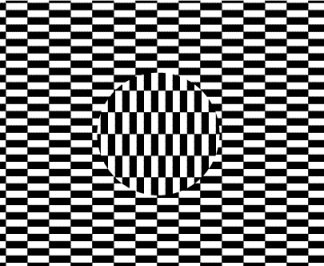
A textured Ouchi Illusion
The Ouchi illusion is a powerful demonstration that static images may produce an illusory movement. One striking aspect is that it makes you feel quite dizzy from trying to compensate for this illusory movement.
The illlusion is is generated by your own eye movements and is a consequence of the aperture problem, which is a fundamental problem in vision science. The aperture problem is the fact that the visual system can only integrate information along the direction of motion, and not perpendicular to it. This is because the visual system is made of a set of filters that are oriented in different directions, and the integration is done by summing the responses of these filters. The aperture problem is a problem because it means that the visual system cannot recover the direction of motion of a contour from the responses of these filters.
Here, we explore variations of this illusion which xwould use textures instead of regular angles using the MotionClouds library. The idea is to use the same texture in the two parts of the image (center vs surround), but to rotate by 90° the texture in the center:
Optimizing the parameters of the texture would help tell us what matters to generate that illusion...
Let's first initialize the notebook:
import numpy as np
import matplotlib.pyplot as plt
fig_width = 10
figsize = (fig_width, fig_width)
install and load the library
%pip install MotionClouds
In particular, we just generate one frame:
def sigmoid(x, # the input
slope=61.803, # this slope is inverse gold times 100
threshold=0.5 # the mean of x
):
# return (x > threshold).astype(np.float)
return 1 / (1 + np.exp(- slope * (x - threshold)))
import MotionClouds as mc
seed = 123456789
N = 512
mc.N_X, mc.N_Y, mc.N_frame = N, N, 1
fx, fy, ft = mc.get_grids(mc.N_X, mc.N_Y, mc.N_frame)
params = dict(theta=0, B_sf=.06, sf_0=.3, B_theta=.1)
params = dict(theta=np.pi/3, B_sf=.5, sf_0=.07, B_theta=.1)
params = dict(theta=0, B_sf=.2, sf_0=.2, B_theta=.25)
params = dict(theta=0, B_sf=.04, sf_0=.2, B_theta=.25)
env = mc.envelope_gabor(fx, fy, ft, **params)
image = mc.rectif(mc.random_cloud(env, seed=seed)).reshape((mc.N_X, mc.N_Y))
image = sigmoid(image)
import matplotlib.pyplot as plt
for key in ['xtick.bottom', 'xtick.labelbottom', 'ytick.left', 'ytick.labelleft']: plt.rcParams[key] = False
%matplotlib inline
fig, ax = plt.subplots(figsize=figsize)
_ = ax.imshow(image, cmap=plt.gray())

define a crop function
The library has a representation of space that we may take advantage of:
fig, ax = plt.subplots(figsize=figsize)
_ = ax.imshow(fx, cmap=plt.gray())
print(fx.min(), fx.max())

We may easily define a central cropping mask:
rho = .2
# mask = ((fx**2 + fy**2) < rho**2).squeeze()
mask = 1-sigmoid((fx**2 + fy**2) - rho**2, slope=1e3, threshold=0).squeeze()
fig, ax = plt.subplots(figsize=figsize)
_ = ax.imshow(mask, cmap=plt.gray())
print(mask.min(), mask.max(), mask.shape)

From this we define a cropping function
def crop_and_merge(image, mask, use_rot=True, use_fill=False, fill=.5):
N_X, N_Y = image.shape
image_fig = image.copy()
if use_rot: image_fig = np.rot90(image_fig)
image_fig = np.roll(image_fig, N_X//4 + int(N_X//2*np.random.rand()), axis=0 ) # roll over one axis
image_fig = np.roll(image_fig, N_Y//4 + int(N_Y//2*np.random.rand()), axis=1 ) # roll over one axis
if use_fill:
return image * (1-mask) + fill * mask
else:
return image * (1-mask) + image_fig * mask
vanilla textured Ouchi illusion
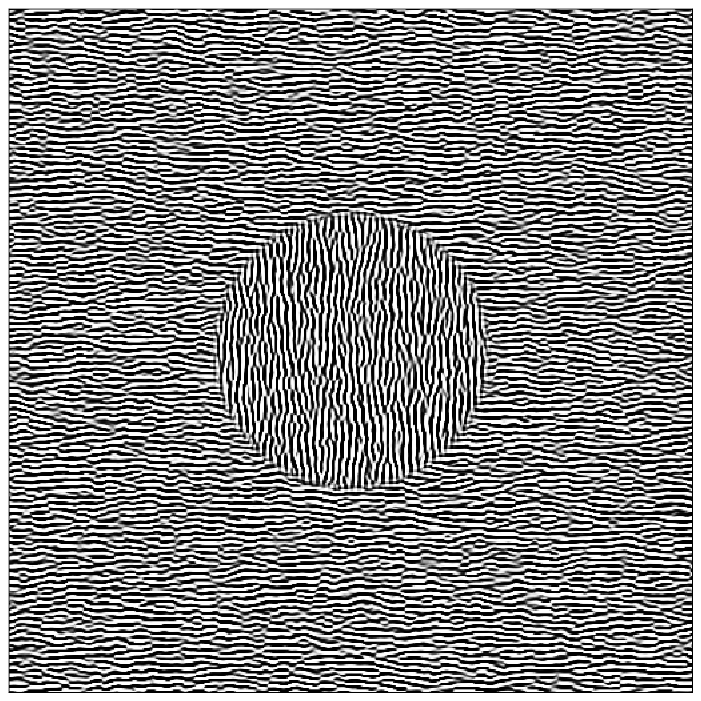
We may now define a function that generates the Ouchi illusion:
fig, ax = plt.subplots(figsize=figsize)
_ = ax.imshow(crop_and_merge(image, mask, use_rot=True), cmap=plt.gray())

fig.savefig('../files/2023-11-29-ouchi-illusion.png', dpi=300, bbox_inches='tight')
A lower frequency produces (in my own eyes) less perceived pulsation and makes the motion aspect of the illusion more powerful:
params_update = params.copy()
params_update.update(sf_0=0.12)
env = mc.envelope_gabor(fx, fy, ft, **params_update)
z = mc.rectif(mc.random_cloud(env, seed=seed))
image_low = z.reshape((mc.N_X, mc.N_Y))
image_low = sigmoid(image_low)
fig, ax = plt.subplots(figsize=figsize)
_ = ax.imshow(crop_and_merge(image_low, mask, use_rot=True), cmap=plt.gray())

and without:
fig, ax = plt.subplots(figsize=figsize)
_ = ax.imshow(crop_and_merge(image, mask, use_rot=False), cmap=plt.gray())

We can also define a first-order figure:
fig, ax = plt.subplots(figsize=figsize)
_ = ax.imshow(crop_and_merge(image, mask, use_fill=True), cmap=plt.gray())

A fun fact is that if you do not threshold the image and have the image in grayscale, the illusion disappears (still with a bit of motion, but not as strong):
params_update = params.copy()
params_update.update(sf_0=0.12)
env = mc.envelope_gabor(fx, fy, ft, **params)
z = mc.rectif(mc.random_cloud(env, seed=seed))
image = z.reshape((mc.N_X, mc.N_Y))
fig, ax = plt.subplots(figsize=figsize)
_ = ax.imshow(crop_and_merge(image, mask, use_rot=True), cmap=plt.gray())

Other masks:
image = mc.rectif(mc.random_cloud(env, seed=seed)).reshape((mc.N_X, mc.N_Y))
image = sigmoid(image)
mask_square = 1-sigmoid(np.abs(fx+fy) + np.abs(fx-fy) - 2*rho, slope=1e3, threshold=0).squeeze()
fig, ax = plt.subplots(figsize=figsize)
_ = ax.imshow(crop_and_merge(image, mask_square, use_rot=True), cmap=plt.gray())

mask_cross = (np.abs(fx) < rho/2) * (np.abs(fy) < rho*2)
mask_cross += (np.abs(fx) < rho*2) * (np.abs(fy) < rho/2)
mask_cross = 1 - (mask_cross>0).squeeze()
fig, ax = plt.subplots(figsize=figsize)
_ = ax.imshow(crop_and_merge(image, mask_cross, use_rot=True), cmap=plt.gray())

mask_bands = (np.sin(2*np.pi*fx*6)>0).squeeze()
fig, ax = plt.subplots(figsize=figsize)
_ = ax.imshow(crop_and_merge(image, mask_bands, use_rot=True), cmap=plt.gray())

mask_chessboard = (np.sin(np.pi*fx*6)*np.sin(np.pi*fy*6)>0).squeeze()
fig, ax = plt.subplots(figsize=figsize)
_ = ax.imshow(crop_and_merge(image, mask_chessboard, use_rot=True), cmap=plt.gray())

changing parameters of the textured Ouchi illusion
We may now define a function that generates the Ouchi illusion:
for sf_0 in params['sf_0'] * np.geomspace(0.1, 3, 7):
print(f'{sf_0=:.3f}')
params_update = params.copy()
params_update.update(sf_0=sf_0)
env = mc.envelope_gabor(fx, fy, ft, **params_update)
z = mc.rectif(mc.random_cloud(env, seed=seed))
image = z.reshape((mc.N_X, mc.N_Y))
image = sigmoid(image)
fig, ax = plt.subplots(figsize=figsize)
_ = ax.imshow(crop_and_merge(image, mask, use_rot=True), cmap=plt.gray())
plt.show()


for B_sf in params['B_sf'] * np.geomspace(0.1, 10, 7):
print(f'{B_sf=:.3f}')
params_update = params.copy()
params_update.update(B_sf=B_sf)
env = mc.envelope_gabor(fx, fy, ft, **params_update)
z = mc.rectif(mc.random_cloud(env, seed=seed))
image = z.reshape((mc.N_X, mc.N_Y))
image = sigmoid(image)
fig, ax = plt.subplots(figsize=figsize)
_ = ax.imshow(crop_and_merge(image, mask, use_rot=True), cmap=plt.gray())
plt.show()


for theta in np.linspace(0, np.pi, 7, endpoint=False):
print(f'{theta=:.3f}')
params_update = params.copy()
params_update.update(theta=theta)
env = mc.envelope_gabor(fx, fy, ft, **params_update)
z = mc.rectif(mc.random_cloud(env, seed=seed))
image = z.reshape((mc.N_X, mc.N_Y))
image = sigmoid(image)
fig, ax = plt.subplots(figsize=figsize)
_ = ax.imshow(crop_and_merge(image, mask, use_rot=True), cmap=plt.gray())
plt.show()


