Static Motion Clouds
Motion Clouds were originally defined as moving textures controlled by a few parameters. The library is also capable to generate a static spatial texture. Herein I describe a solution to generate a single static frame.
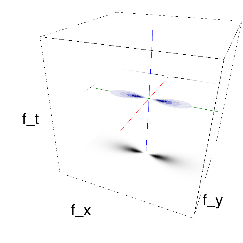
There are multiple solutions, and the simplest is perhaps to generate a movie that does not move. This means that the mean velocity $(V_X, V_Y)$ is null $=(0, 0)$ but also that there is no noise in the definition of the speed plane. This is defined by $B_V=0$, that is, that all the energy is concentrated on the spped plane:
import MotionClouds as mc
fx, fy, ft = mc.get_grids(mc.N_X, mc.N_Y, mc.N_frame)
name = 'static'
env = mc.envelope_gabor(fx, fy, ft, V_X=0., V_Y=0., B_V=0)
mc.figures(env, name)
mc.in_show_video(name)
 |
||
 |
||
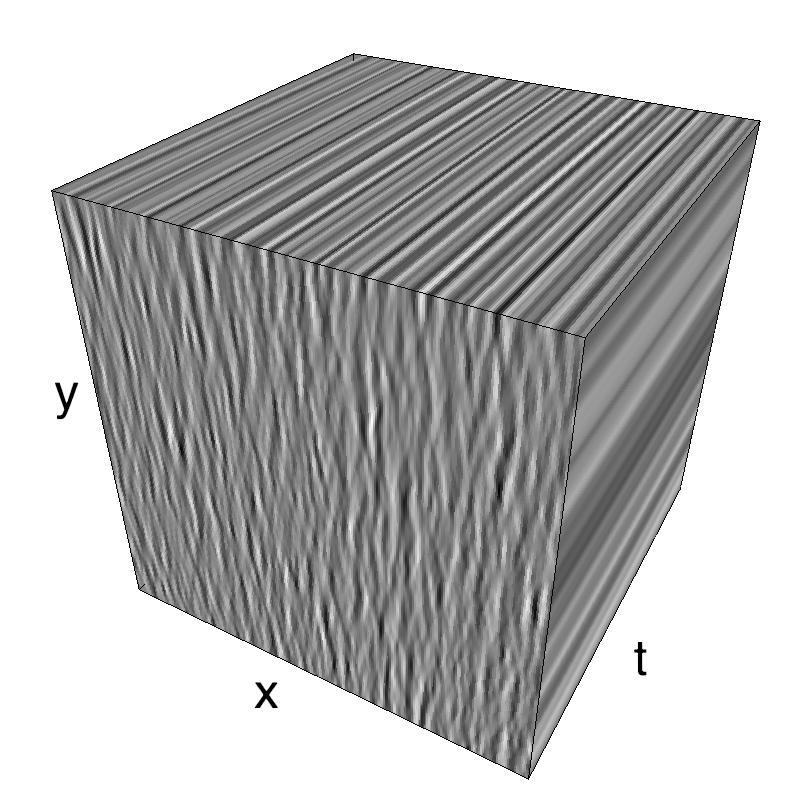
As such, all frames are the same and it suffices to take one of them.
Note that as a matter of fact there is a "mathematical issue" here: if we define $B_V = 0$ in our implementation we need to take care of the fact that the formula for the Gaussian doest not give a "dividion by zero" error. The MotionClouds code takes this possibility into accountin the mc.envelope_speed function:
help(mc.envelope_speed)
However, this solution is not the most elegant and one could also just state that N_frame is 1 (that is, that the movie consists of only one frame).
The library is made such that this will also work in this slightly degenerate mode:
mc.N_frame=1
fx, fy, ft = mc.get_grids(mc.N_X, mc.N_Y, mc.N_frame)
name = 'static'
env = mc.envelope_gabor(fx, fy, ft, V_X=0., V_Y=0., B_V=0)
z = mc.rectif(mc.random_cloud(env))
print(z.shape)
z = z.reshape((mc.N_X, mc.N_Y))
Note that in that case, you need to reshape your matrix to one dimension. Using this numpy array, you can now simply plot it:
import matplotlib.pyplot as plt
%matplotlib inline
fig, ax = plt.subplots(figsize=(10,10))
_ = ax.imshow(z.T, cmap=plt.gray())

a simple application: defining a set of stimuli with different orientation bandwidths
import numpy as np
import MotionClouds as mc
import matplotlib.pyplot as plt
downscale = 1
fx, fy, ft = mc.get_grids(mc.N_X/downscale, mc.N_Y/downscale, 1)


N_theta = 6
bw_values = np.pi*np.logspace(-2, -5, N_theta, base=2)
fig_width = 21


fig, axs = plt.subplots(1, N_theta, figsize=(fig_width, fig_width/N_theta))
for i_ax, B_theta in enumerate(bw_values):
    mc_i = mc.envelope_gabor(fx, fy, ft, V_X=0., V_Y=0., B_V=0, theta=np.pi/2, B_theta=B_theta)
    im = mc.random_cloud(mc_i)

    axs[i_ax].imshow(im[:, :, 0], cmap=plt.gray())
    axs[i_ax].text(5, 29, r'$B_\theta=%.1f$°' % (B_theta*180/np.pi), color='white', fontsize=32)
    axs[i_ax].set_xticks([])
    axs[i_ax].set_yticks([])
plt.tight_layout()
fig.subplots_adjust(hspace = .0, wspace = .0, left=0.0, bottom=0., right=1., top=1.)

#import os
#fig.savefig(os.path.join('../figs', 'orientation_tuning.png'))
