Embedding a trajectory in noise
Motion detection has many functions, one of which is the potential localization of the biomimetic camouflage seen in this video. Can we test this in the lab by using synthetic textures such as MotionClouds?
However, by construction, MotionClouds have no spatial structure and it seems interesting to consider more complex trajectories. Following a previous post, we design a trajectory embedded in noise.
Can you spot the motion ? from left to right or reversed ?
(For a more controlled test, imagine you fixate on the top left corner of each movie.)
(Upper row is coherent, lower row uncoherent / Left is -> Right column is <-)
Let's start with the classical Motion Cloud:
name = 'trajectory'
%matplotlib inline
import matplotlib.pyplot as plt
import os
import numpy as np
import MotionClouds as mc
fx, fy, ft = mc.get_grids(mc.N_X, mc.N_Y, mc.N_frame)

mc.figpath = '../files/2018-11-13-testing-more-complex'
if not(os.path.isdir(mc.figpath)): os.mkdir(mc.figpath)
Some default parameters for the textons used here:
opts = dict(sf_0=0.04, B_sf=0.02, B_theta=np.inf, B_V=1.1, V_X=2.)
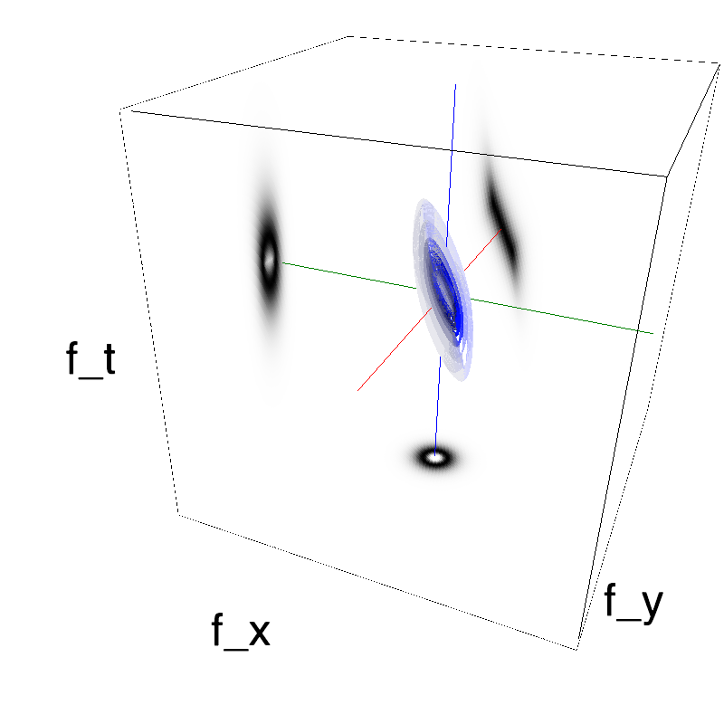
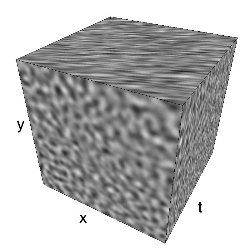
First defining a dense,stationary noise with an horizontal drift:
name_ = name + '_dense'
seed = 42
mc1 = mc.envelope_gabor(fx, fy, ft, **opts)
mc.figures(mc1, name_, seed=seed, figpath=mc.figpath)
mc.in_show_video(name_, figpath=mc.figpath)
 |
||
 |
||
The information is distributed densely in space and time.
one definition of a trajectory
It is also possible to show the impulse response ("texton") corresponding to this particular texture (be patient to see a full period):
name_ = name + '_impulse'
seed = 42
mc1 = mc.envelope_gabor(fx, fy, ft, **opts)
mc.figures(mc1, name_, seed=seed, impulse=True, figpath=mc.figpath)
mc.in_show_video(name_, figpath=mc.figpath)
 |
||
 |
||
To generate a trajectory, we should just convolve this impulse response to a trajectory defined as a binary profile in space and time:
name_ = name + '_straight'
seed = 42
x, y, t = fx+.5, fy+.5, ft+.5 # trick to use fourier coordinates to get spatial coordinates
width_y, width_x = 1/mc.N_X, 1/mc.N_Y
t0, t1 = .375, .625
x0 = .25 #np.random.rand() * (1 - opts['V_X'] * (t1-t0)) # makes sure the trajectory does not wrap across the border
y0 = np.random.rand()
events = 1. * (np.abs(y - y0) < width_y)* (np.abs(x - x0 - opts['V_X']*(t-t0)) < width_x) * (t > t0 ) * (t < t1)
fig, ax = plt.subplots(1, 1, figsize=(15, 15))
ax.imshow(events.mean(axis=1))
ax.set_xlabel('Time')
ax.set_ylabel('X-axis');

mc1 = mc.envelope_gabor(fx, fy, ft, **opts)
mc.figures(mc1, name_, seed=seed, events=events, figpath=mc.figpath)
mc.in_show_video(name_, figpath=mc.figpath)
 |
||
 |
||
To replicate the work from Watamaniuk, McKee and colleagues, we replicate the same motion but where we keep the motion energy while shuffling the coherence:
name_ = name + '_shuffled'
N_folds = 8
N_traj = int((t1-t0)*mc.N_frame) // N_folds
N_start = int(t0*mc.N_frame)
folding = np.random.permutation(N_folds)
events_shuffled = events.copy()
for i_fold in range(N_folds):
    S0, S1 = (N_start+folding[i_fold]*N_traj), (N_start+(folding[i_fold]+1)*N_traj)
    N0, N1 = (N_start+i_fold*N_traj), (N_start+(i_fold+1)*N_traj)
    if False:
        nx = int(np.random.rand()*mc.N_Y)
    else:
        nx = 0 # do not shuffle on the y-axis
    ny = int(np.random.rand()*mc.N_Y)
    events_shuffled[:, :, S0:S1] = np.roll(np.roll(events[:, :, N0:N1], nx, axis=0), ny, axis=1)

fig, ax = plt.subplots(1, 1, figsize=(15, 15))
ax.imshow(events_shuffled.mean(axis=1))
ax.set_xlabel('Time')
ax.set_ylabel('X-axis');

mc1 = mc.envelope_gabor(fx, fy, ft, **opts)
mc.figures(mc1, name_, seed=seed, events=events_shuffled, figpath=mc.figpath)
mc.in_show_video(name_, figpath=mc.figpath)
 |
||
 |
||
addition of a the trajectory to the incoherent noise
It is now possible to add this trajectory to any kind of background, such as a background texture of the same "texton" but with a null average motion:
def overlay(movie1, movie2, rho, do_linear=False):
    if do_linear:
        return rho*movie1+(1-rho)*movie2
    else:
        movie1, movie2 = rho*(2.*movie1-1), 2.*movie2-1
        movie = np.zeros_like(movie1)
        mask = np.abs(movie1) > np.abs(movie2)
        movie[mask] = movie1[mask]
        movie[1-mask] = movie2[1-mask]
        return .5 + .5*movie
a more memory-efficient version of the above:
def overlay(movie1, movie2, rho, do_linear=False):
    if do_linear:
        return rho*movie1+(1-rho)*movie2
    else:
        movie1, movie2 = rho*(2.*movie1-1), 2.*movie2-1
        movie = movie1 * (np.abs(movie1) > np.abs(movie2)) + movie2 * (np.abs(movie1) <= np.abs(movie2))
        #return .5 + .5*movie
        return 1. * (movie > 0.)
        #seuil = .1
        #return .5 + .5 * (-1. * (movie < -seuil) +  1. * (movie > seuil))
        #return  .5 + .5* np.tan(4.*movie)
mc1 = mc.envelope_gabor(fx, fy, ft, **opts)
movie_coh = mc.rectif(mc.random_cloud(mc1, seed=seed, events=events))
opts_ = opts.copy()
opts_.update(V_X=0)
mc0 = mc.envelope_gabor(fx, fy, ft, **opts_)
movie_unc = mc.rectif(mc.random_cloud(mc0, seed=seed+1))
name_ = name + '_overlay'
rho_coh = .9
mc.anim_save(overlay(movie_coh, movie_unc, rho_coh), os.path.join(mc.figpath, name_))
mc.in_show_video(name_, figpath=mc.figpath)
name_ = name + '_overlay_difficult'
rho_coh = .5
mc.anim_save(overlay(movie_coh, movie_unc, rho_coh), os.path.join(mc.figpath, name_))
mc.in_show_video(name_, figpath=mc.figpath)
Though it is difficult to find the coherent pattern in a single frame, one detects it thanks to its coherent motion.
name_ = name + '_overlay_shuffled'
movie_coh_shuffled = mc.rectif(mc.random_cloud(mc1, seed=seed, events=events_shuffled))
rho_coh = .9
mc.anim_save(overlay(movie_coh_shuffled, movie_unc, rho_coh), os.path.join(mc.figpath, name_))
mc.in_show_video(name_, figpath=mc.figpath)
name_ = name + '_overlay_difficult_shuffled'
rho_coh = .5
mc.anim_save(overlay(movie_coh_shuffled, movie_unc, rho_coh), os.path.join(mc.figpath, name_))
mc.in_show_video(name_, figpath=mc.figpath)
trying out different directions
rho_coh = .9
name_ = name + '_overlay_reversed'
mc.anim_save(overlay(movie_coh[::-1, :, :], movie_unc, rho_coh), os.path.join(mc.figpath, name_))
mc.in_show_video(name_, figpath=mc.figpath)
name_ = name + '_overlay_shuffled_reversed'
mc.anim_save(overlay(movie_coh_shuffled[::-1, :, :], movie_unc, rho_coh), os.path.join(mc.figpath, name_))
mc.in_show_video(name_, figpath=mc.figpath)
some book keeping for the notebook
%load_ext watermark
%watermark
%load_ext watermark
%watermark -i -h -m -v -p MotionClouds,numpy,pillow,imageio  -r -g -b