Testing more complex trajectories
MotionClouds may be considered as a control stimulus - it seems more interesting to consider more complex trajectories.
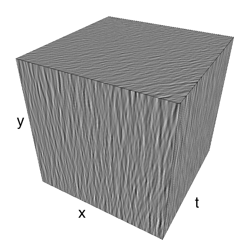
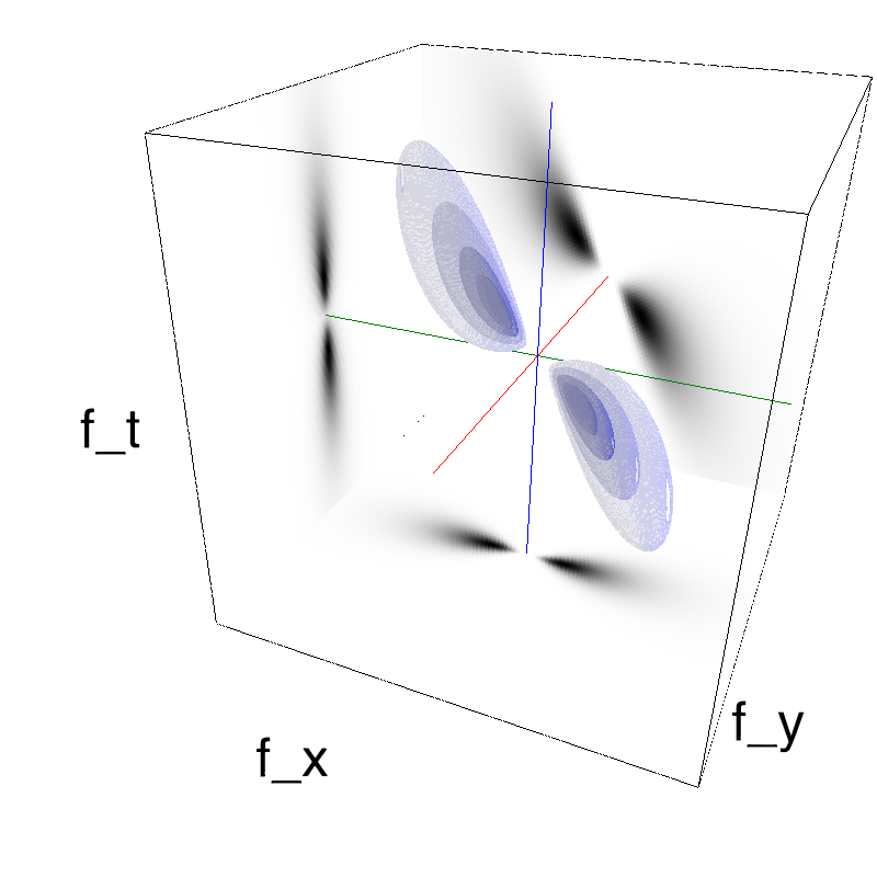
Let's start with the classical Motion Cloud:
name = 'trajectory'
import os
import numpy as np
import MotionClouds as mc
fx, fy, ft = mc.get_grids(mc.N_X, mc.N_Y, mc.N_frame)

mc.figpath = '../files/2018-01-16-testing-more-complex'
if not(os.path.isdir(mc.figpath)): os.mkdir(mc.figpath)
name_ = name + '_dense'
seed = 42
mc1 = mc.envelope_gabor(fx, fy, ft)
mc.figures(mc1, name_, seed=seed, figpath=mc.figpath)
mc.in_show_video(name_, figpath=mc.figpath)
The information is distributed densely in space and time.
one definition of a trajectory
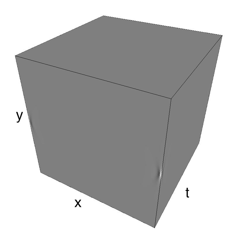
It is also possible to show the impulse response ("texton") corresponding to this particular texture (be patient to see a full period):
name_ = name + '_impulse'
seed = 42
mc1 = mc.envelope_gabor(fx, fy, ft)
mc.figures(mc1, name_, seed=seed, impulse=True, figpath=mc.figpath)
mc.in_show_video(name_, figpath=mc.figpath)
To generate a trajectory, we should just convolve this impulse response to a trajectory defined as a binary profile in space and time:
name_ = name + '_straight'
seed = 42
x, y, t = fx+.5, fy+.5, ft+.5
width_y, width_x = 0.01, 0.005
events = 1. * (np.abs(y - .5) < width_y )* (np.abs(x - t) < width_x )
mc1 = mc.envelope_gabor(fx, fy, ft)
mc.figures(mc1, name_, seed=seed, events=events, figpath=mc.figpath)
mc.in_show_video(name_, figpath=mc.figpath)
It is possible to make this trajectory noisy:
name_ = name + '_noisy'
noise_x = 0.02
noise = noise_x * np.random.randn(1, 1, mc.N_frame)
events = 1. * (np.abs(y - .5) < width_y )* (np.abs(x + noise - t) < width_x )
mc1 = mc.envelope_gabor(fx, fy, ft)
mc.figures(mc1, name_, seed=seed, events=events, figpath=mc.figpath)
mc.in_show_video(name_, figpath=mc.figpath)
Finally, it is possible to make the amplitude of the texton change as a function of time:
name_ = name + '_noisier'
noise = noise_x * np.random.randn(1, 1, mc.N_frame)
events = 1. * (np.abs(y - .5) < width_y )* (np.abs(x + noise - t) < width_x )
A_noise_x = 0.02
A_noise = A_noise_x * np.random.randn(1, 1, mc.N_frame)
phase_noise = 2 * np.pi * np.random.rand(1, 1, mc.N_frame)
A_noise = np.cumsum(A_noise, axis=-1) / np.sqrt(t+1)
phase_noise = np.cumsum(phase_noise, axis=-1)
mc1 = mc.envelope_gabor(fx, fy, ft)
mc.figures(mc1, name_, seed=seed, events=A_noise*np.exp(phase_noise*1j)*events, figpath=mc.figpath)
mc.in_show_video(name_, figpath=mc.figpath)
addition of a trajectory to the incoherent noise
It is now possible to add this trajectory to any kind of background, such as a background texture of the same "texton" but with a null average motion:
name_ = name + '_overlay'
movie_coh = mc.rectif(mc.random_cloud(mc1, seed=seed, events=A_noise*np.exp(phase_noise*1j)*events))
mc0 = mc.envelope_gabor(fx, fy, ft, V_X=0)
movie_unc = mc.rectif(mc.random_cloud(mc0, seed=seed+1))
rho_coh = .9
mc.anim_save(rho_coh*movie_coh+(1-rho_coh)*movie_unc, os.path.join(mc.figpath, name_))
mc.in_show_video(name_, figpath=mc.figpath)
name_ = name + '_overlay_difficult'
rho_coh = .5
mc.anim_save(rho_coh*movie_coh+(1-rho_coh)*movie_unc, os.path.join(mc.figpath, name_))
mc.in_show_video(name_, figpath=mc.figpath)
Though it is difficult to find the coherent pattern in a single frame, one detects it thanks to its coherent motion (see work from Watamaniuk, McKee and colleagues).
some book keeping for the notebook
%load_ext version_information
%version_information numpy, matplotlib, MotionClouds


