Motion Plaids

Laurent Perrinet

2014-10-20 17:50

MotionPlaids : from MotionClouds components to a plaid-like stimulus¶

In [1]:

import numpy as np
import MotionClouds as mc
downscale = 2
fx, fy, ft = mc.get_grids(mc.N_X/downscale, mc.N_Y/downscale, mc.N_frame/downscale)
name = 'MotionPlaid'

mc.figpath = '../files/2014-10-20_MotionPlaids'
import os
if not(os.path.isdir(mc.figpath)): os.mkdir(mc.figpath)

Plaids are usually created by adding two moving gratings (the components) to form a new simulus (the pattern). Such stimuli are crucial to understand how for instance information about motion is represented and processed and its neural mechanisms have been extensively studied notably by Anthony Movshon at the NYU. One shortcomming is the fact that these are created by components which created interference patterns when they are added (as in a Moiré pattern). The question remains to know if everything that we know about components vs pattern processing comes from these interference patterns or reaaly by the processing of the two componenents as a whole. As such, Motion Clouds are ideal candidates because they are generated with random phases: by construction, there should not be any localized interference between components. Let's verfy that:

Defintion of parameters:

In [2]:

theta1, theta2, B_theta = np.pi/4., -np.pi/4., np.pi/32

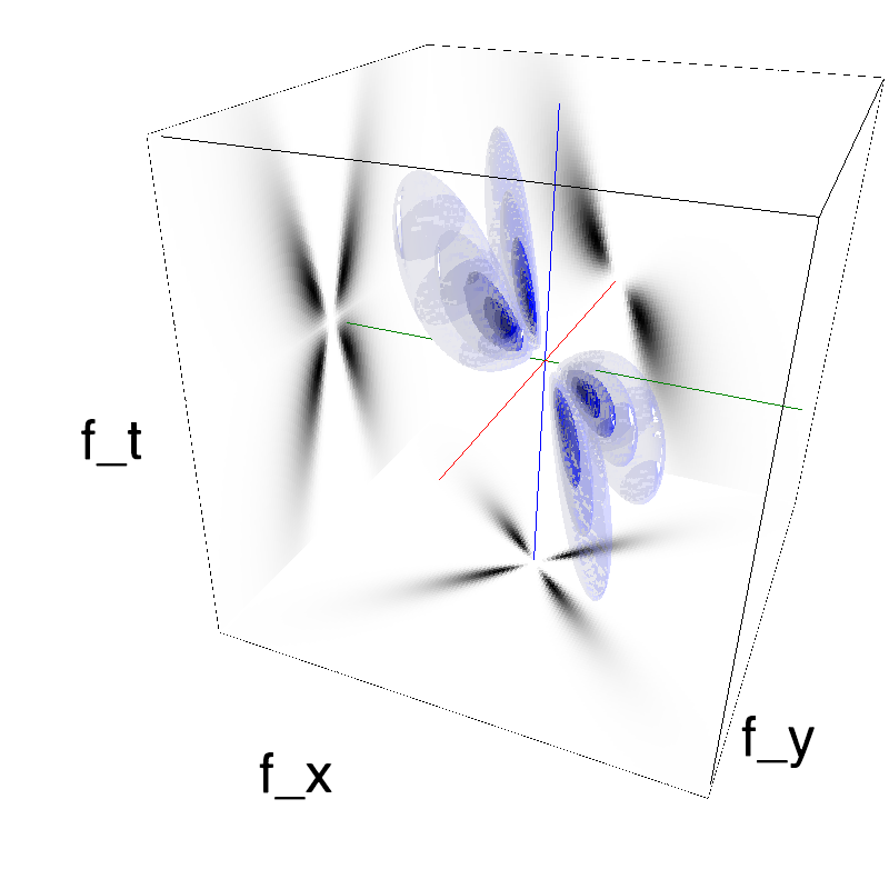
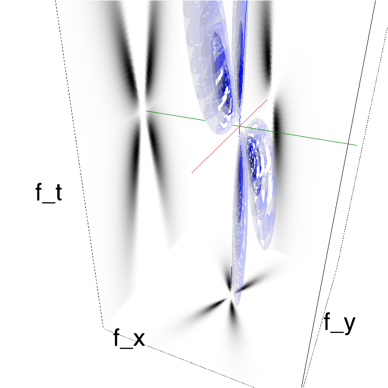
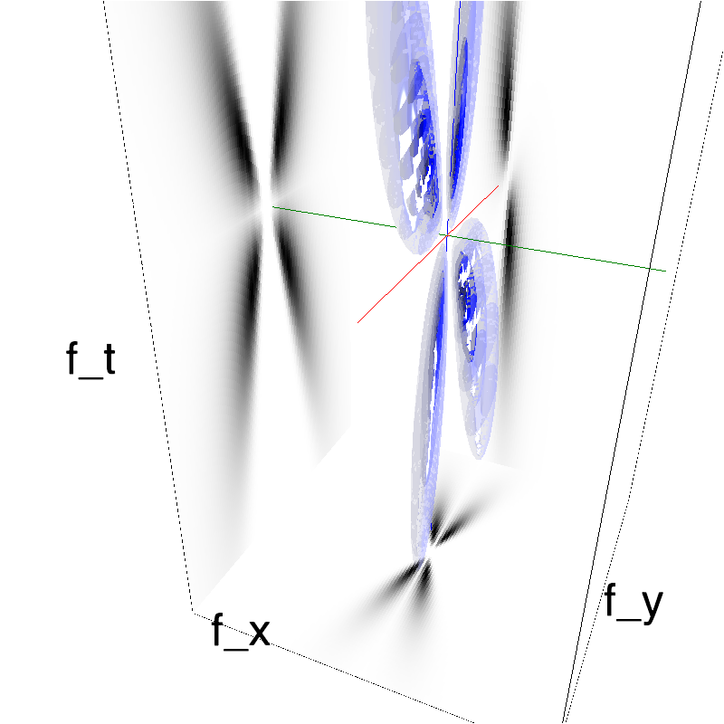
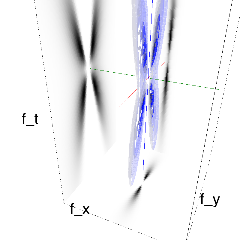
This figure shows how one can create MotionCloud stimuli that specifically target component and pattern cell. We show in the different lines of this table respectively: Top) one motion cloud component (with a strong selectivity toward the orientation perpendicular to direction) heading in the upper diagonal Middle) a similar motion cloud component following the lower diagonal Bottom) the addition of both components: perceptually, the horizontal direction is predominant.

In [3]:

print( mc.in_show_video.__doc__)


    Columns represent isometric projections of a cube. The left column displays
    iso-surfaces of the spectral envelope by displaying enclosing volumes at 5
    different energy values with respect to the peak amplitude of the Fourier spectrum.
    The middle column shows an isometric view of the faces of the movie cube.
    The first frame of the movie lies on the x-y plane, the x-t plane lies on the
    top face and motion direction is seen as diagonal lines on this face (vertical
    motion is similarly see in the y-t face). The third column displays the actual
    movie as an animation.

    Given a name, displays the figures corresponding to the Fourier spectra, the
    stimulus cubes and movies within the notebook.

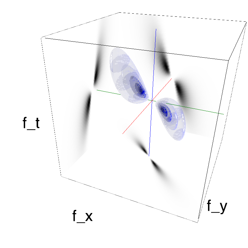
Component one:

In [4]:

diag1 = mc.envelope_gabor(fx, fy, ft, theta=theta1, V_X=np.cos(theta1), V_Y=np.sin(theta1), B_theta=B_theta)
name_ = name + '_comp1'
mc.figures(diag1, name_, seed=12234565, figpath=mc.figpath)
mc.in_show_video(name_, figpath=mc.figpath)

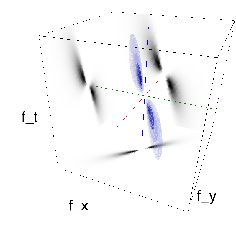
Component two:

In [5]:

diag2 = mc.envelope_gabor(fx, fy, ft, theta=theta2, V_X=np.cos(theta2), V_Y=np.sin(theta2), B_theta=B_theta)
name_ = name + '_comp2'
mc.figures(diag2, name_, seed=12234565, figpath=mc.figpath)
mc.in_show_video(name_, figpath=mc.figpath)

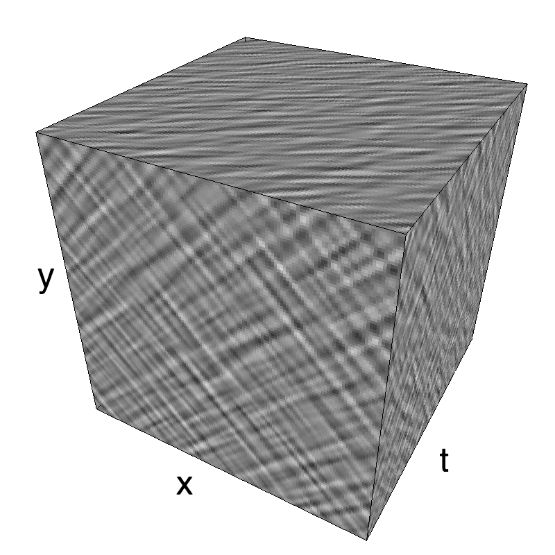
The pattern is the sum of the two components:

In [6]:

name_ = name
mc.figures(diag1 + diag2, name, seed=12234565, figpath=mc.figpath)
mc.in_show_video(name_, figpath=mc.figpath)

A grid of plaids shows switch from transparency to pattern motion¶

Script done in collaboration with Jean Spezia.

In [7]:

import os
import numpy as np
import MotionClouds as mc

name = 'MotionPlaid_9x9'
if mc.check_if_anim_exist(name):
    B_theta = np.pi/32
    N_orient = 9
    downscale = 4
    fx, fy, ft = mc.get_grids(mc.N_X//downscale, mc.N_Y//downscale, mc.N_frame//downscale)
    mov = mc.np.zeros(((N_orient*mc.N_X//downscale), (N_orient*mc.N_X//downscale), mc.N_frame//downscale))
    i = 0
    j = 0
    for theta1 in np.linspace(0, np.pi/2, N_orient)[::-1]:
        for theta2 in np.linspace(0, np.pi/2, N_orient):
            diag1 = mc.envelope_gabor(fx, fy, ft, theta=theta1, V_X=np.cos(theta1), V_Y=np.sin(theta1), B_theta=B_theta)
            diag2 = mc.envelope_gabor(fx, fy, ft, theta=theta2, V_X=np.cos(theta2), V_Y=np.sin(theta2), B_theta=B_theta)
            mov[(i)*mc.N_X//downscale:(i+1)*mc.N_X//downscale, (j)*mc.N_Y//downscale : (j+1)*mc.N_Y//downscale, :] = mc.random_cloud(diag1 + diag2, seed=1234)
            j += 1
        j = 0
        i += 1
    mc.anim_save(mc.rectif(mov, contrast=.99), os.path.join(mc.figpath, name))

In [8]:

mc.in_show_video(name, figpath=mc.figpath)

As in (Rust, 06) we show in this table the concatenation of a table of 9x9 MotionPlaids where the angle of the components vary on respectively the horizontal and vertical axes.
The diagonal from the bottom left to the top right corners show the addition of two component MotionClouds of similar direction: They are therefore also intance of the same Motion Clouds and thus consist in a single component.
As one gets further away from this diagonal, the angle between both component increases, as can be seen in the figure below. Note that first and last column are different instance of similar MotionClouds, just as first and last lines in in the table.

A parametric exploration on MotionPlaids¶

In [9]:

N_orient = 8
downscale = 2
fx, fy, ft = mc.get_grids(mc.N_X/downscale, mc.N_Y/downscale, mc.N_frame)
theta = 0
for dtheta in np.linspace(0, np.pi/2, N_orient):
    name_ = name + 'dtheta_' + str(dtheta).replace('.', '_')
    diag1 = mc.envelope_gabor(fx, fy, ft, theta=theta + dtheta, V_X=np.cos(theta + dtheta), V_Y=np.sin(theta + dtheta), B_theta=B_theta)
    diag2 = mc.envelope_gabor(fx, fy, ft, theta=theta - dtheta, V_X=np.cos(theta - dtheta), V_Y=np.sin(theta - dtheta), B_theta=B_theta)
    mc.figures(diag1 + diag2, name_, seed=12234565, figpath=mc.figpath)
    mc.in_show_video(name_, figpath=mc.figpath)

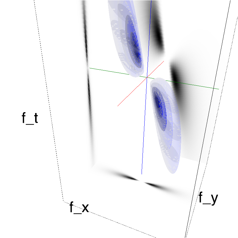
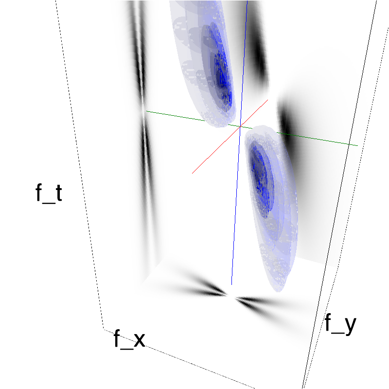
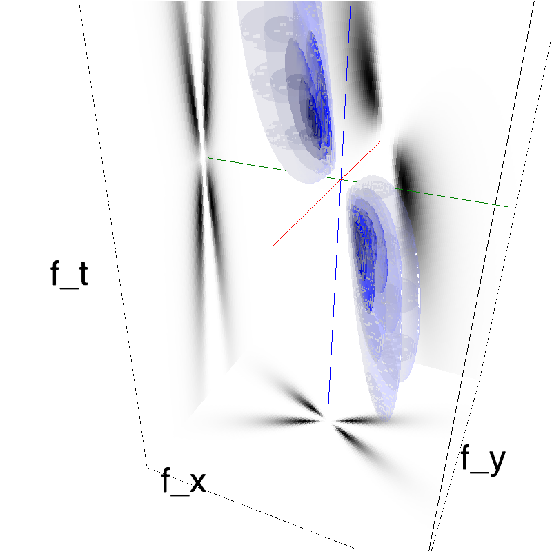
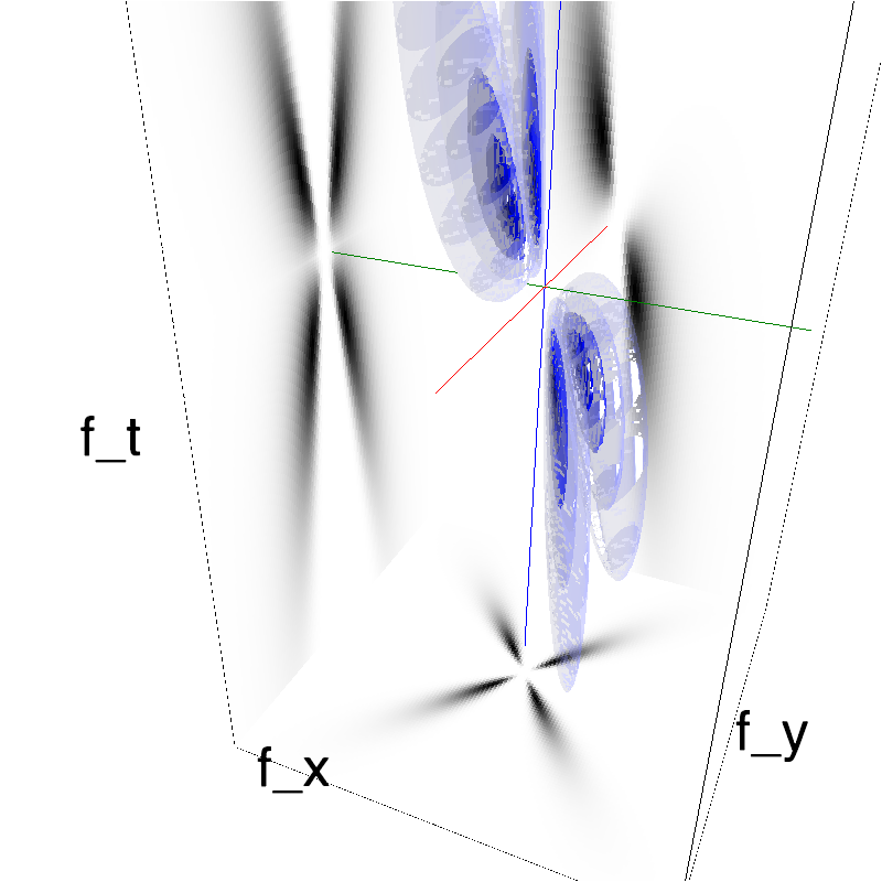
For clarity, we display MotionPlaids as the angle between both component increases from 0 to pi/2.
Left column displays iso-surfaces of the spectral envelope by displaying enclosing volumes at 5 different energy values with respect to the peak amplitude of the Fourier spectrum.
Right column of the table displays the actual movie as an animation.