Aperture Problem
SlippingClouds: MotionClouds for exploring the aperture problem
import numpy as np
import MotionClouds as mc

fx, fy, ft = mc.get_grids(mc.N_X, mc.N_Y, mc.N_frame)
name = 'SlippingClouds'

import os
mc.figpath = '../files/2014-10-20_Aperture-Problem'
if not(os.path.isdir(mc.figpath)): os.mkdir(mc.figpath)

B_sf = .3
B_theta = np.pi/32
theta1, theta2 = 0., 0.
diag = mc.envelope_gabor(fx, fy, ft, theta=theta2, V_X=np.cos(theta1), V_Y=np.sin(theta1), B_sf=B_sf, B_theta=B_theta)
name_ = name + '_iso'
mc.figures(diag, name_, seed=12234565, figpath=mc.figpath)
mc.in_show_video(name_, figpath=mc.figpath)
 |
||
 |
||
theta1, theta2 = 0., np.pi/4.
diag = mc.envelope_gabor(fx, fy, ft, theta=theta2, V_X=np.cos(theta1), V_Y=np.sin(theta1), B_sf=B_sf, B_theta=B_theta)
name_ = name + '_diag'
mc.figures(diag, name_, seed=12234565, figpath=mc.figpath)
mc.in_show_video(name_, figpath=mc.figpath)
 |
||
 |
||
theta1, theta2 = 0., np.pi/2.
diag = mc.envelope_gabor(fx, fy, ft, theta=theta2, V_X=np.cos(theta1), V_Y=np.sin(theta1), B_sf=B_sf, B_theta=B_theta)
name_ = name + '_contra'
mc.figures(diag, name_, seed=12234565, figpath=mc.figpath)
mc.in_show_video(name_, figpath=mc.figpath)
 |
||
 |
||
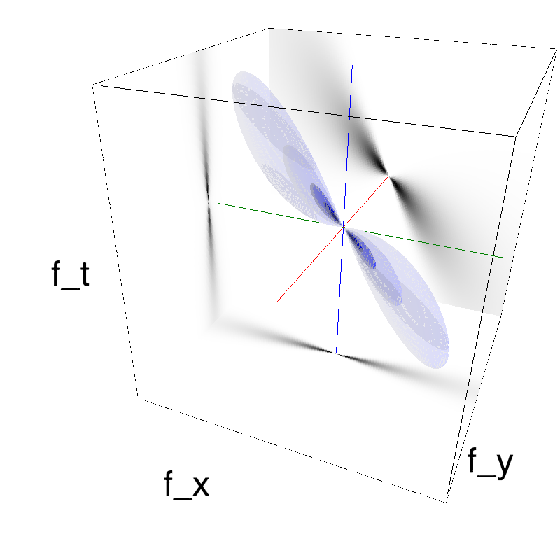
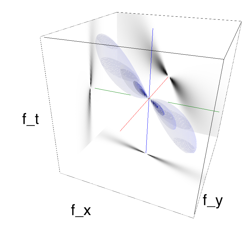
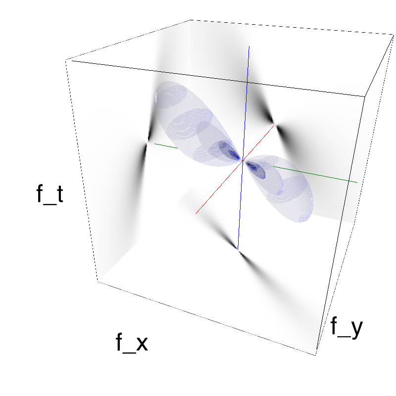
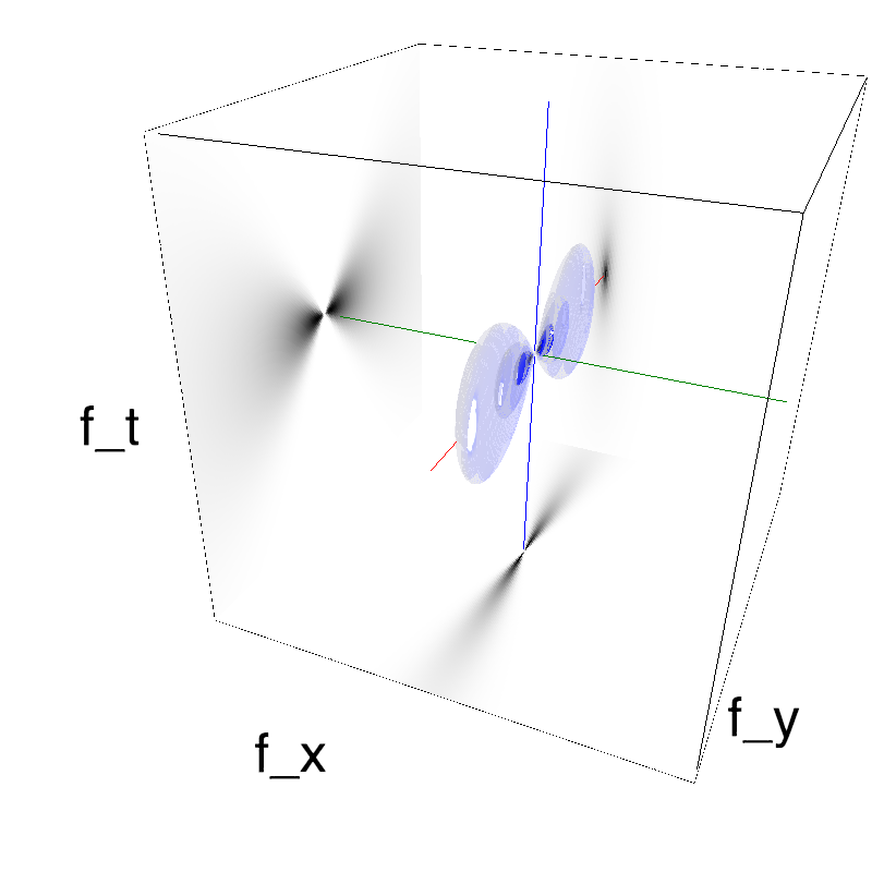
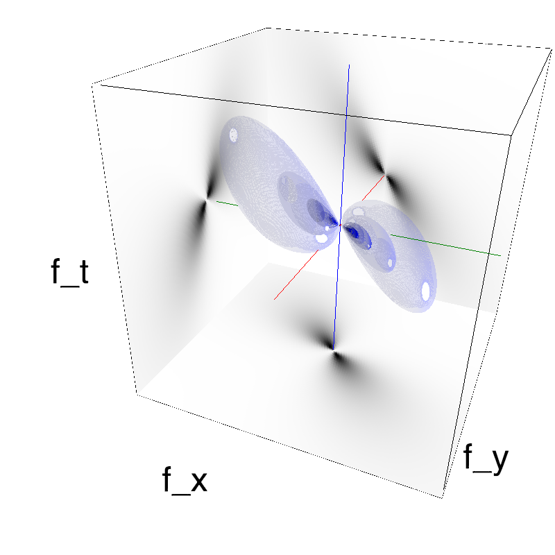
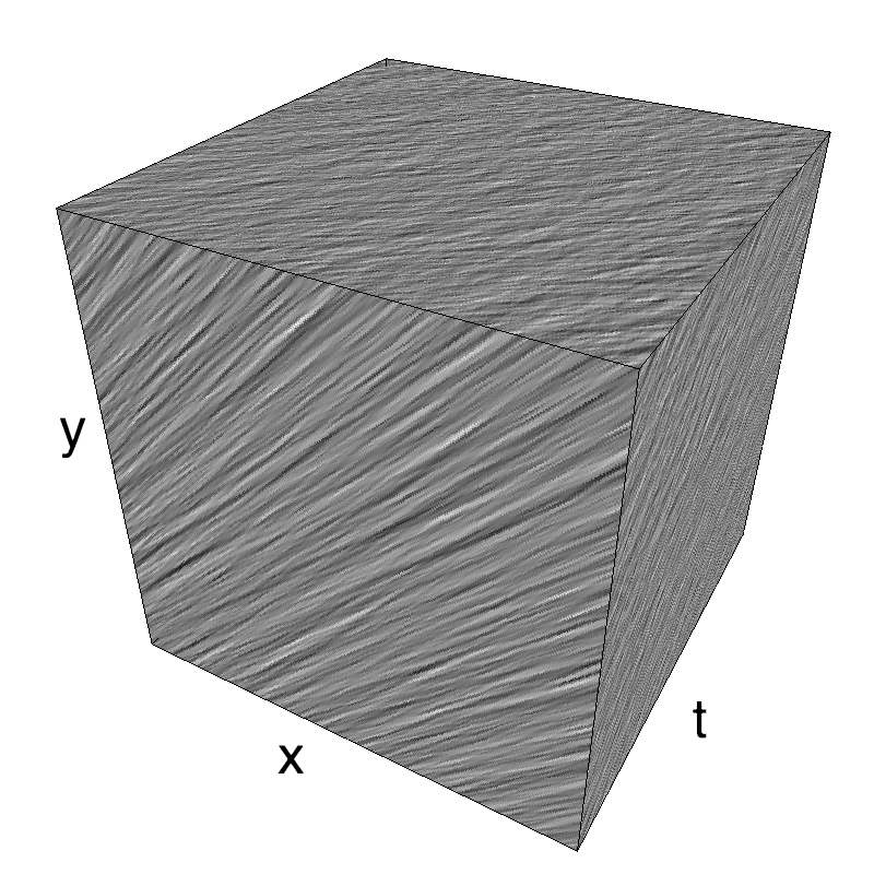
This figure shows how one can create MotionCloud stimuli that have specific direction and orientation which are not necessarily perpendicular, components "slipping" relative to the motion.
We generate MotionClouds components with a strong selectivity toward one orientation. We show in different lines of this table respectively: Top) orientation perpendicular to orientation as in the standard case with a line, Middle) a 45° difference between both, Bottom) orientation and direction are parallel.
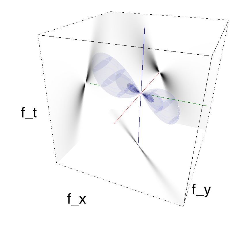
We created the aperture problem without any aperture! This can be shown by looking at envelopes in the Fourier space. To best infer motion, you would look fro the best speed plane that would go through each envelope. If these envelopes are rather tight, there are many different speed planes that can go through this envelope: motion is ambiguous.
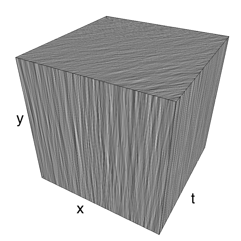
Columns represent isometric projections of a cube. The left column displays iso-surfaces of the spectral envelope by displaying enclosing volumes at 5 different energy values with respect to the peak amplitude of the Fourier spectrum. The middle column shows an isometric view of the faces of the movie cube.
The first frame of the movie lies on the x-y plane, the x-t plane lies on the top face and motion direction is seen as diagonal lines on this face (vertical motion is similarly see in the y-t face). The third column displays the actual movie as an animation.
exploring different slipping angles
N_orient = 8
#downscale= 2
#fx, fy, ft = mc.get_grids(mc.N_X/downscale, mc.N_Y/downscale, mc.N_frame)
theta = 0
for dtheta in np.linspace(0, np.pi/2, N_orient):
    name_ = name + '_dtheta_' + str(dtheta).replace('.', '_')
    theta1, theta2, B_theta = 0., np.pi/2., np.pi/32
    diag = mc.envelope_gabor(fx, fy, ft, theta=theta+dtheta, V_X=np.cos(theta), V_Y=np.sin(theta), B_sf=B_sf, B_theta=B_theta)
    mc.figures(diag, name_, seed=12234565, figpath=mc.figpath)
    mc.in_show_video(name_, figpath=mc.figpath)
 |
||
 |
||
 |
||
 |
||
 |
||
 |
||
 |
||
 |
||
 |
||
 |
||
 |
||
 |
||
 |
||
 |
||
 |
||
 |
||
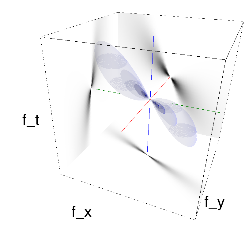
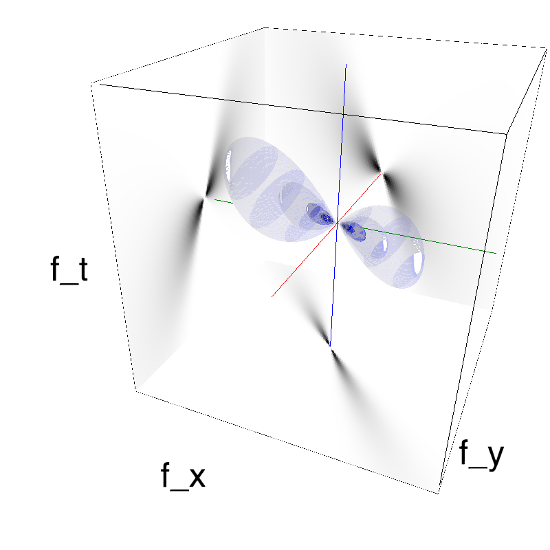
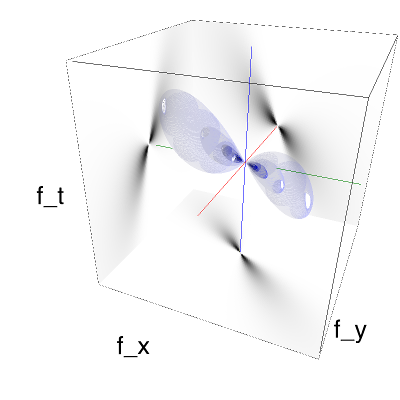
We display SlippingClouds with different angle between direction and orientation.
Left column displays iso-surfaces of the spectral envelope by displaying enclosing volumes at 5 different energy values with respect to the peak amplitude of the Fourier spectrum.
Right column of the table displays the actual movie as an animation.
manipulating different ambiguities
N_test = 8
#downscale= 2
#fx, fy, ft = mc.get_grids(mc.N_X/downscale, mc.N_Y/downscale, mc.N_frame)
theta = 0
dtheta = np.pi/4
for B_theta_ in np.pi/8/np.arange(1, N_test+1):#np.linspace(0, np.pi/8, N_test)[1:]:
    name_ = name + '_B_theta_' + str(B_theta_).replace('.', '_')
    theta1, theta2, B_theta = 0., np.pi/2., np.pi/32
    diag = mc.envelope_gabor(fx, fy, ft, theta=theta+dtheta, V_X=np.cos(theta), V_Y=np.sin(theta), B_sf=B_sf, B_theta=B_theta_)
    mc.figures(diag, name_, seed=12234565, figpath=mc.figpath)
    mc.in_show_video(name_, figpath=mc.figpath)
 |
||
 |
||
 |
||
 |
||
 |
||
 |
||
 |
||
 |
||
 |
||
 |
||
 |
||
 |
||
 |
||
 |
||
 |
||
 |
||
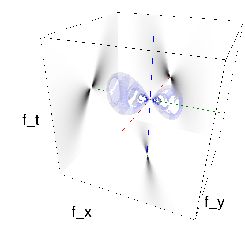
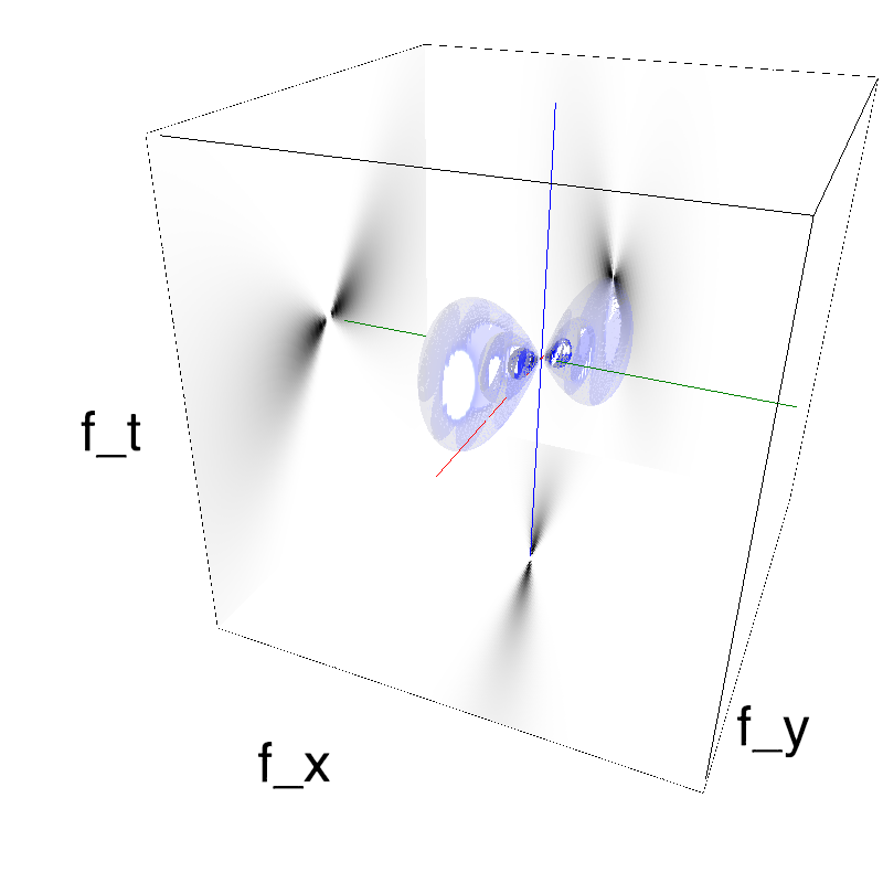
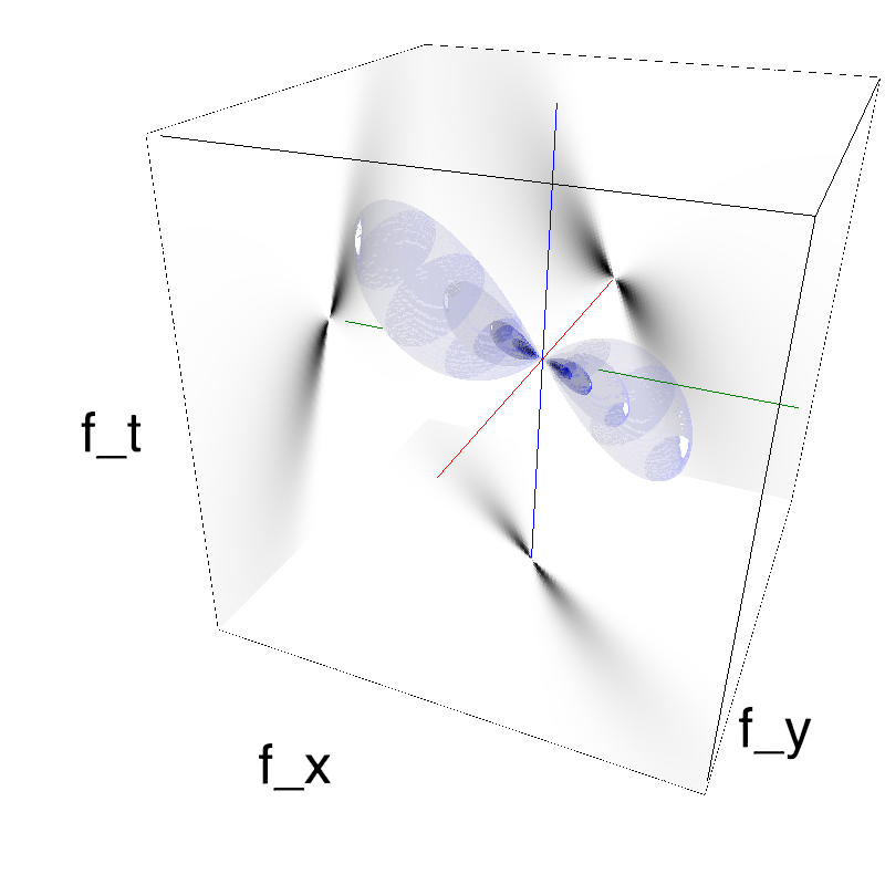
The ambiguity in !SlippingClouds can be manipualted by changing B_theta for a given B_V.
Left column displays iso-surfaces of the spectral envelope by displaying enclosing volumes at 5 different energy values with respect to the peak amplitude of the Fourier spectrum.
Right column of the table displays the actual movie as an animation.
some book keeping for the notebook
%load_ext version_information
%version_information numpy, scipy, matplotlib, MotionClouds