Implementing a retinotopic transform using `grid_sample` from pyTorch
Implementing a retinotopic transform using grid_sample from pyTorch
The grid_sample transform is a powerful function which allows to transform any input image into a new topology. It is notably used in Spatial Transformer Networks for instance to learn CNN to be invariant to affine transforms. We used it recently in a publication What You See Is What You Transform: Foveated Spatial Transformers as a Bio-Inspired Attention Mechanism by Ghassan Dabane et al.
The use of grid_sample can b etedious and here, we show how to use it to create a log-polar transform of the image and create the following figure:
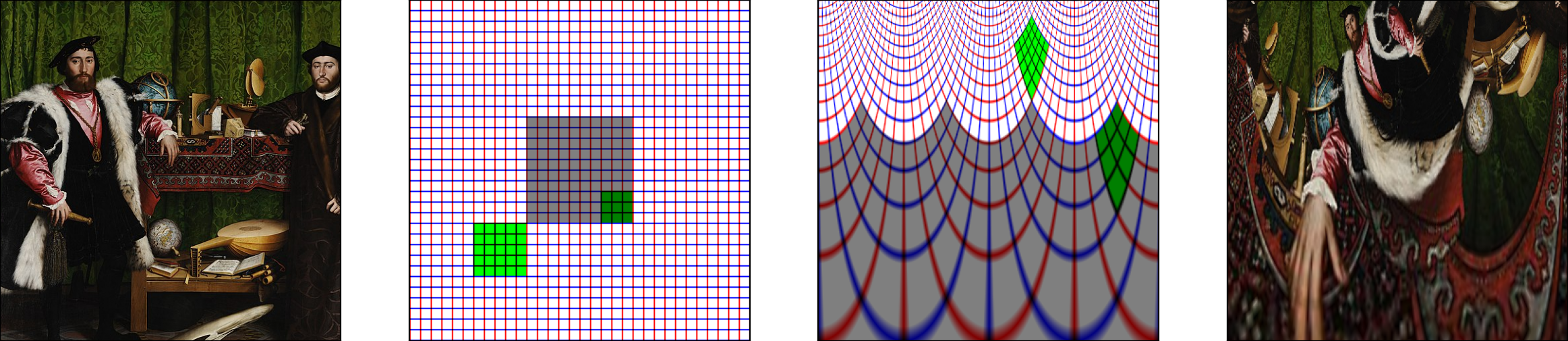
A picture (extract from the painting "The Ambassadors" by Hans Holbein the Younger can be represented on a regular grid represented by vertical (red) and horizontal (blue) lines. Retinotopy transforms this grid, and in particular the area representing the fovea (shaded gray) is over-represented. Applied to the original image of the portrait, the image is strongly distorted and represents more finally the parts under the axis of sight (here the mouth).
Let's first initialize the notebook :
import os

import numpy as np
import torch
torch.set_printoptions(precision=3, linewidth=140, sci_mode=False)
import torch.nn.functional as F

import matplotlib.pyplot as plt
fig_width = 15
dpi = 'figure'
dpi = 200
opts_savefig = dict(dpi=dpi, bbox_inches='tight', pad_inches=0, edgecolor=None)

image_size_grid = 257
definition of the grid
Let's first define a first grid as a set of points defined in absolute coordinates between $-1$ and $1$, and define the corresponding meshgrid:
image_size_az, image_size_el = 360, 360
rs_ = torch.logspace(0, -4, image_size_az, base=2)
ts_ = torch.linspace(-torch.pi, torch.pi, image_size_el+1)[:-1]

grid_xs = torch.outer(rs_, -torch.cos(ts_))
grid_ys = torch.outer(rs_, torch.sin(ts_))
grid_xs.shape, grid_ys.shape
These are then formated in the right format to be used by the function:
center_x, center_y = 0., 0. # defines the fixation point's center in absolute coordinates
logPolar_grid = torch.stack((grid_xs-center_x, grid_ys-center_y), 2)
logPolar_grid = logPolar_grid.unsqueeze(0) # add batch dim
logPolar_grid.shape
logPolar_grid.min()
# F.grid_sample?
application to a synthetic image
We define a synthetic image to illustrate the transform, it consists of white pixels, red verticals and blue horizontals, regularly spaced:
image_grid_size = 8
image_grid_tens = torch.ones((3, image_size_grid, image_size_grid)).float()
image_grid_tens[0:2, ::image_grid_size, :] = 0
image_grid_tens[1:3, :, ::image_grid_size] = 0
fovea_size = 5
image_grid_tens[[0, 2],
                int(image_size_grid//2+image_grid_size*fovea_size/2.5):int(image_size_grid//2+image_grid_size*fovea_size),
                int(image_size_grid//2+image_grid_size*fovea_size/2.5):int(image_size_grid//2+image_grid_size*fovea_size),
                ] = 0
image_grid_tens[[0, 2],
                int(image_size_grid//2+image_grid_size*fovea_size):int(image_size_grid//2+image_grid_size*fovea_size*2),
                int(image_size_grid//2-image_grid_size*fovea_size*2):int(image_size_grid//2-image_grid_size*fovea_size),
                ] = 0
image_grid_tens[:, (image_size_grid//2-image_grid_size*fovea_size):(image_size_grid//2+image_grid_size*fovea_size), (image_size_grid//2-image_grid_size*fovea_size):(image_size_grid//2+image_grid_size*fovea_size)] *= .5
image_grid_tens.shape, image_grid_tens.unsqueeze(0).shape
to display it, we need to transform the torch format to a numpy / matplotlib compatible one, which can be first tested on a MWE (minimal working example) using torch.movedim:
torch.movedim(torch.randn(1, 2, 3), (0, 1, 2), (1, 2, 0)).shape
this can be done on the image in a few lines:
image_grid = image_grid_tens.squeeze(0)
# swap from C, H, W (torch) to H, W, C (numpy)
image_grid = torch.movedim(image_grid, (1, 2, 0), (0, 1, 2))
image_grid = image_grid.numpy()
image_grid.shape
so that we can display the synthetic image:
fig, ax = plt.subplots(figsize=(fig_width, fig_width))
ax.imshow(image_grid)
ax.plot(image_size_grid//2, image_size_grid//2, 'r+', markersize=40, markeredgewidth=5)
ax.set_xticks([])
ax.set_yticks([])
fig.set_facecolor(color='white')

Let's transform the image of the grid:
image_grid_ret_tens = F.grid_sample(image_grid_tens.unsqueeze(0).float(), logPolar_grid, align_corners=False, padding_mode='border')
image_grid_tens.shape, logPolar_grid.shape, image_grid_ret_tens.shape
and transform it back to numpy:
image_grid_ret_tens = image_grid_ret_tens.squeeze(0)
# swap from C, H, W (torch) to H, W, C (numpy)
image_grid_ret_tens = torch.movedim(image_grid_ret_tens, (1, 2, 0), (0, 1, 2))
image_grid_ret = image_grid_ret_tens.numpy()
image_grid_ret /= image_grid_ret.max()
image_grid_ret.shape
to then display the retinotopic transform of the grid image:
fig, ax = plt.subplots(figsize=(fig_width, fig_width))
ax.imshow(image_grid_ret)
ax.set_xticks([])
ax.set_yticks([])
fig.set_facecolor(color='white')

application to a natural image
Let's load an image by extracting a part from the painting "The Ambassadors" by Hans Holbein the Younger:
image_size = 513
image_url = 'https://upload.wikimedia.org/wikipedia/commons/8/88/Hans_Holbein_the_Younger_-_The_Ambassadors_-_Google_Art_Project.jpg'
image_url = 'https://upload.wikimedia.org/wikipedia/commons/thumb/8/88/Hans_Holbein_the_Younger_-_The_Ambassadors_-_Google_Art_Project.jpg/608px-Hans_Holbein_the_Younger_-_The_Ambassadors_-_Google_Art_Project.jpg'
# from PIL import ImageFile
# ImageFile.LOAD_TRUNCATED_IMAGES = True
# import imageio
import imageio.v2 as imageio

im_shift_X, im_shift_Y = 0, 27
image = imageio.imread(image_url)[im_shift_X:im_shift_X+image_size, im_shift_Y:im_shift_Y+image_size, :] / 255
image.max()
and display it:
fig, ax = plt.subplots(figsize=(fig_width, fig_width))
ax.imshow(image)
ax.set_xticks([])
ax.set_yticks([])
fig.set_facecolor(color='white')

to use it in the function, we need to transform the numpy format to a torch compatible one, which can be first tested on a MWE (minimal working example):
torch.movedim(torch.randn(1, 2, 3), (1, 2, 0), (0, 1, 2)).shape
this now looks like:
image_tens = torch.from_numpy(image)
# swap from H, W, C (numpy) to C, H, W (torch)
image_tens = torch.movedim(image_tens, (0, 1, 2), (1, 2, 0))
image.shape, image_tens.shape
Let's transform the image:
image_ret_tens = F.grid_sample(image_tens.unsqueeze(0).float(), logPolar_grid, align_corners=False, padding_mode='border')
image_ret_tens.shape
and transform it back to numpy:
image_ret_tens = image_ret_tens.squeeze(0)
# swap from C, H, W (torch) to H, W, C (numpy)
image_ret_tens = torch.movedim(image_ret_tens, (1, 2, 0), (0, 1, 2))
image_ret = image_ret_tens.numpy()
and display it:
fig, ax = plt.subplots(figsize=(fig_width, fig_width))
ax.imshow(image_ret)
ax.set_xticks([])
ax.set_yticks([])
fig.set_facecolor(color='white')

summary
fig, axs = plt.subplots(1, 4, figsize=(fig_width, fig_width))
axs[0].imshow(image)
axs[1].imshow(image_grid)
axs[2].imshow(image_grid_ret)
axs[3].imshow(image_ret)
for ax in axs:
    ax.set_xticks([])
    ax.set_yticks([])
fig.set_facecolor(color='white')
fname = '../files/2023-02-02-implementing-a-retinotopic-transform-using-grid_sample-from-pytorch'
fig.savefig(fname + '.png', dpi=200, bbox_inches='tight', pad_inches=0, edgecolor=None)
# fig.savefig(fname + '_dpi800.png', dpi=800, bbox_inches='tight', pad_inches=0, edgecolor=None)
# fig.savefig(fname + '_dpi1500.png', dpi=1500, bbox_inches='tight', pad_inches=0, edgecolor=None)

Appendix: version of the libraries that were used
%load_ext watermark
%watermark -i -h -m -v -p numpy,torch,matplotlib  -r -g -b