Dreamachine
It's at the MIAM (Miam Musée International des Arts Modestes) in Sète, France, that I could for the first time experience really the Dreamachine. It's an optical system which consists of a central light which is periodically occluded by a rotating (cardboard?) cylinder.
The magic of it is that the frequency of occlusion is around $12$ Hz, an important resonant state for sensory system. For the first time, I could really try it out at the MIAM - the important point being to close your lids and rest quiet while looking at the stroboscopic light source. Surprisingly, you see the emergence of "psychedelic patterns" (of course, less than in hippie's movies) yet of the order of the color pattern that may arise in Benham's Disk.
It's difficult to reproduce this pattern on a screen, yet it is still possible to give an impression of it. The goal is here :
-
to generate a complex visual stimulation flickering on average at $12$ Hz
-
to project it on a retinotopic space to maximise the "psychedelic" effect
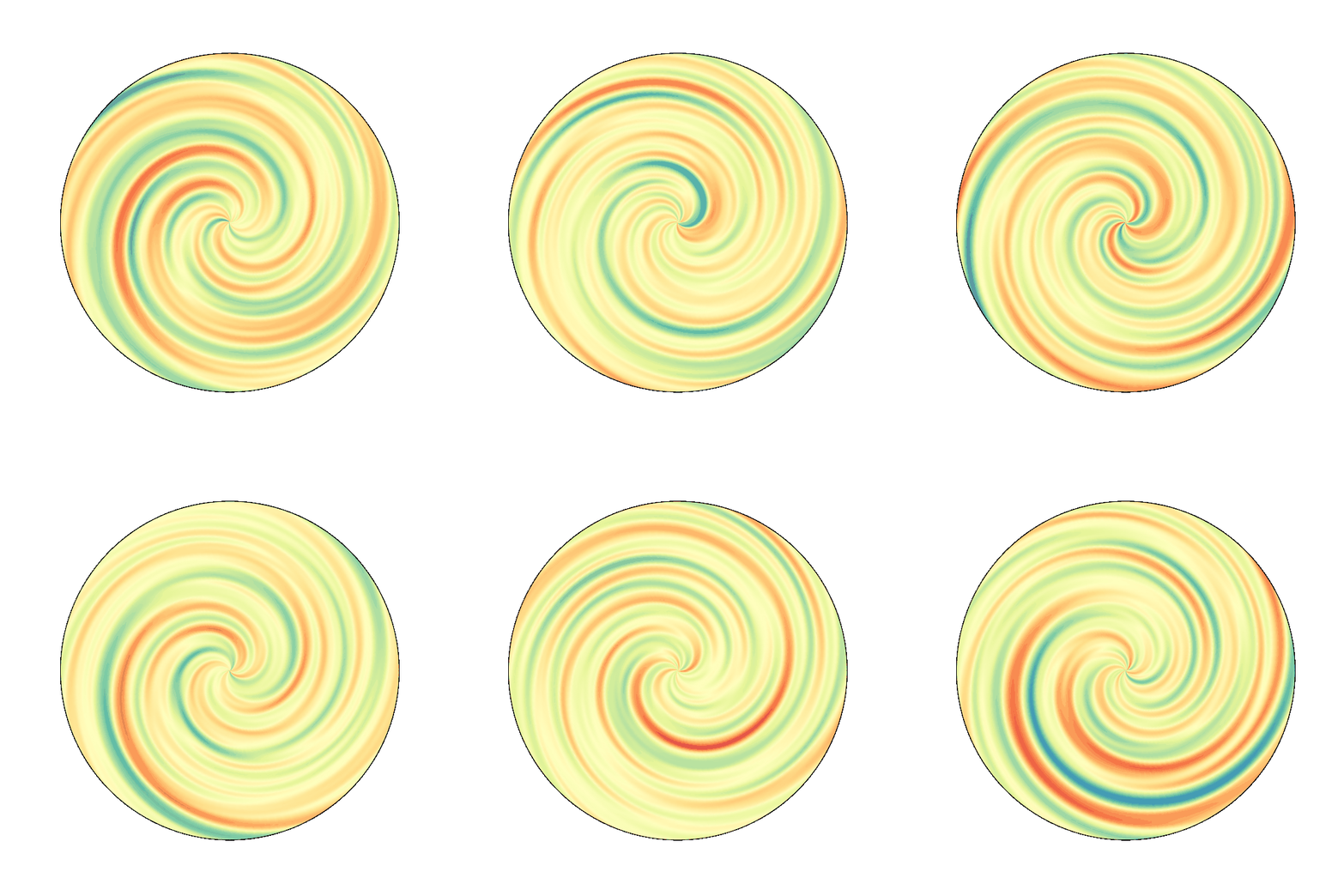
Let's first initialize the notebook:
from __future__ import division, print_function
import numpy as np
np.set_printoptions(precision=6, suppress=True)
import os
%matplotlib inline
%config InlineBackend.figure_format='retina'
#%config InlineBackend.figure_format = 'svg'
import matplotlib.pyplot as plt
phi = (np.sqrt(5)+1)/2
fig_width = 10
figsize = (fig_width, fig_width/phi)
# https://docs.python.org/3/library/warnings.html#warning-filter
import warnings
warnings.simplefilter("ignore")

%load_ext autoreload
%autoreload 2
a flickering motion cloud
A simple way to generate a flickering stimulus is to combine two sinusiods going in two opposite directions, following :
$$ \sin(\omega_x \cdot x + \omega_t \cdot v \cdot t) + \sin(\omega_x \cdot x - \omega_t \cdot v \cdot t) = 2\cdot \cos(\omega_x \cdot x) \cdot \cos(\omega_t \cdot v \cdot t) $$
A first solution is to use an existing library for generating band-pass filtered noise, with a parameterization which fits well natural scenes:
import os
name = 'alpha'
DOWNSCALE = 2
import MotionClouds as mc
mc.figpath = '../files/2022-01-30-dreamachine'
os.makedirs(mc.figpath, exist_ok=True)
Let's explore parameters:
mc.envelope_gabor?
To find that which will best will what we wish to do:
T_movie = 2.4 # period in seconds
fps = 60 # frames per second
sf_0 = 0.05 # spatial frequency per period
TF_0 = 12.  # peak temporal frequency
seed = 1234
N_X, N_Y, N_frame = 256//DOWNSCALE, 256//DOWNSCALE, int(T_movie*fps)
print(f'{N_X=}, {N_Y=}, {N_frame=}')
fx, fy, ft = mc.get_grids(N_X, N_Y, N_frame)

tf_0 = TF_0/fps # temporal frequency per period
V_X = tf_0 / sf_0
B_V = 0.12
theta = 0
B_theta = .1
print(f'{V_X=}, {sf_0=}, {tf_0=}')
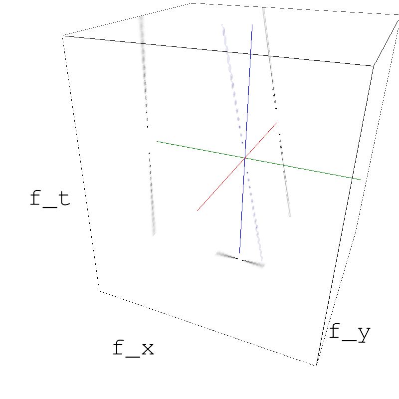
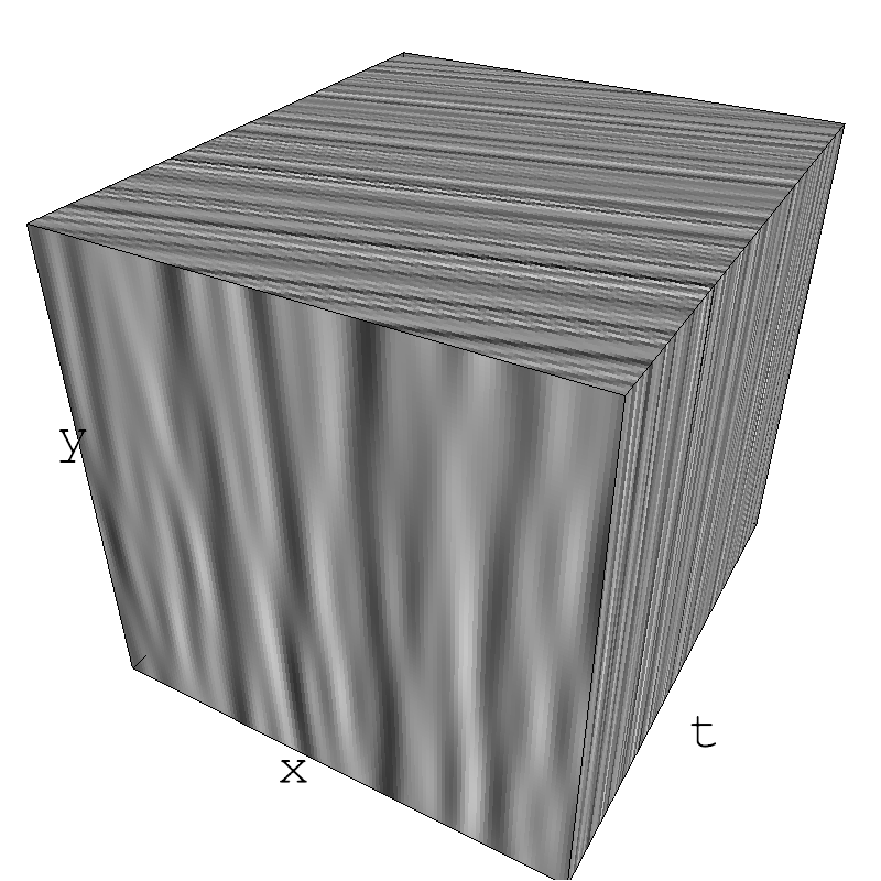
z_1 = mc.envelope_gabor(fx, fy, ft, V_X=V_X, sf_0=sf_0, B_V=B_V, theta=theta, B_theta=B_theta)
name_ = name + '_1'
#mc.anim_save(movie_1, os.path.join(mc.figpath, name_))
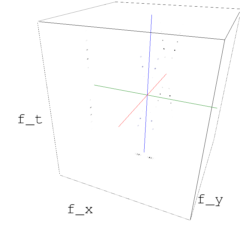
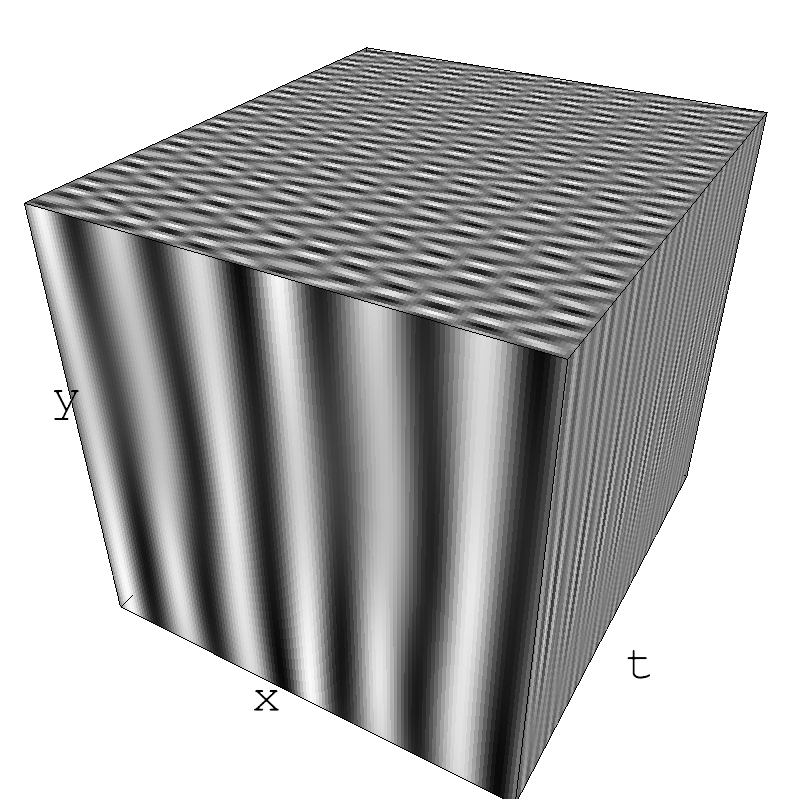
mc.figures(z_1, name_, figpath=mc.figpath, seed=seed)
mc.in_show_video(name_, figpath=mc.figpath)
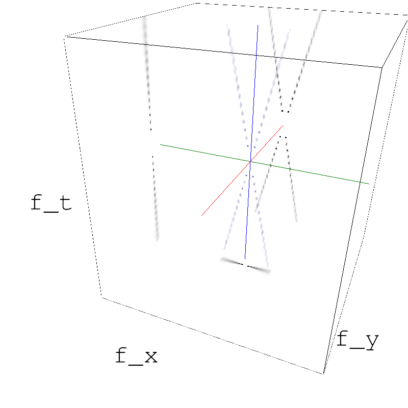
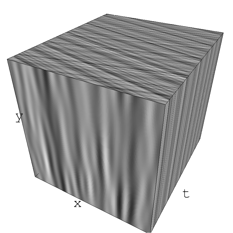
z_2 = mc.envelope_gabor(fx, fy, ft, V_X=-V_X, sf_0=sf_0, B_V=B_V, theta=theta, B_theta=B_theta)
z_12 = z_1 + z_2
#movie_2 = mc.rectif(mc.random_cloud(z_2))
#movie_12 = mc.rectif(movie_1 + movie_2)

name_ = name + '_12'
#mc.anim_save(movie_12, os.path.join(mc.figpath, name_))
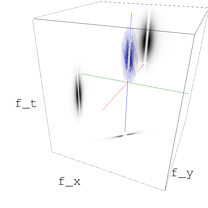
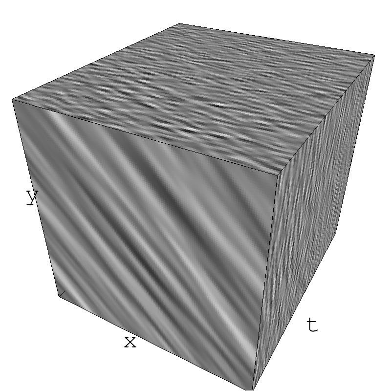
mc.figures(z_12, name_, figpath=mc.figpath, seed=seed)
mc.in_show_video(name_, figpath=mc.figpath)
The combination of both wavec indeedd generates a flickering effect, but to increase it, let's make the wave more sinusoid-like by making the envelope more "tight":
tightness = 8.
z_1 = mc.envelope_gabor(fx, fy, ft, V_X=V_X, sf_0=sf_0, B_sf=0.1/tightness, B_V=B_V/tightness, theta=theta, B_theta=B_theta)
z_2 = mc.envelope_gabor(fx, fy, ft, V_X=-V_X, sf_0=sf_0, B_sf=0.1/tightness, B_V=B_V/tightness, theta=theta, B_theta=B_theta)

z_12 = z_1 + z_2

name_ = name + '_12_tight'
#mc.anim_save(movie_12, os.path.join(mc.figpath, name_))
mc.figures(z_12, name_, figpath=mc.figpath, seed=seed)
mc.in_show_video(name_, figpath=mc.figpath)
This indeed looks better, but we may also follow a simpler route by generating our custom envelope.
custom cloud
Let's inspire us by the function which defines the enveloppe :
mc.frequency_radius?
and to define a custom one
tf_0
ft.min(), ft.max()
B_sf = .05
B_tf = .1
B_theta = .1
theta = np.pi*(3 - np.sqrt(5)) # https://en.wikipedia.org/wiki/Golden_angle
def envelope_alpha(fx, fy, ft, tf_0=tf_0, B_tf=B_tf, sf_0=sf_0, B_sf=B_sf, theta=theta, B_theta=B_theta):
    #f_radius = mc.frequency_radius(fx, fy, ft, ft_0=1.0, clean_division=True)
    ft_ = ft + 1.0*(ft==0.) # to avoid numerical errors
    #env = 1./np.abs(ft_)*np.exp(-.5*(np.log((ft_/tf_0)**2))/((np.log((tf_0+B_tf)/tf_0))**2))
    env = np.exp(-.5*(ft_-tf_0)**2/B_tf**2)
    env *= mc.envelope_orientation(fx, fy, ft, theta=theta, B_theta=B_theta)
    env *= mc.envelope_radial(fx, fy, ft, sf_0=sf_0, B_sf=B_sf)

    return env
z_pure = envelope_alpha(fx, fy, ft, tf_0=tf_0, B_tf=B_tf, B_sf=B_sf, theta=theta, B_theta=B_theta)

name_ = name + '_pure'
mc.figures(z_pure, name_, figpath=mc.figpath, recompute=True, seed=seed)
mc.in_show_video(name_, figpath=mc.figpath)
retinotopic mapping
We can directly acess the movie as a 3D ndarray:
movie_pure = mc.rectif(mc.random_cloud(z_pure, seed=seed))
One may want to project it on retinotopic coordinates to give a psychedelic effect...
Following this answer, it's pretty easy to take one image and to project it to a retinotopic map. In our case, there are no color, so it's even easier...
movie_pure_ = np.zeros((movie_pure.shape[0], movie_pure.shape[1]+1, movie_pure.shape[2]))
movie_pure_[:, :-1, :] = movie_pure
movie_pure_[:, -1, :] = movie_pure[:, 0, :]
movie_pure = movie_pure_
# get coordinates of boxes in the mesh :
phi = np.linspace(0, 2*np.pi, movie_pure.shape[1])
r = np.linspace(0, 1, movie_pure.shape[0])
Phi, R = np.meshgrid(phi, r)
fig, ax = plt.subplots(1, 1, figsize=(fig_width, fig_width), subplot_kw=dict(polar=True))
# https://matplotlib.org/3.1.1/api/_as_gen/matplotlib.pyplot.pcolormesh.html
# https://matplotlib.org/devdocs/gallery/images_contours_and_fields/pcolormesh_grids.html
m = ax.pcolormesh(Phi, R, movie_pure[:, :, 0], shading='gouraud', vmin=movie_pure.min(), vmax=movie_pure.max(),
                  edgecolors='none', linewidth=0, cmap=plt.gray())
ax.set_xticks([])
ax.set_yticks([]);
Let's sature the grayscale values to give it a more natural look:
movie_pure_bw = np.tanh(2*movie_pure)
fig, ax = plt.subplots(1, 1, figsize=(fig_width, fig_width), subplot_kw=dict(polar=True))
#fig.subplots_adjust(bottom=0.4, left=.3, right=0.6, top=0.6);
# https://matplotlib.org/3.1.1/api/_as_gen/matplotlib.pyplot.pcolormesh.html
# https://matplotlib.org/devdocs/gallery/images_contours_and_fields/pcolormesh_grids.html
m = ax.pcolormesh(Phi, R, movie_pure_bw[:, :, 0], shading='gouraud',
                  vmin=movie_pure_bw.min(), vmax=movie_pure_bw.max(),
                  edgecolors='none', cmap=plt.gray())
#ax.margins(y=-0.2)
ax.set_xticks([])
ax.set_yticks([]);
DREAMACHINE videos
Following a previous post, we can make a one-cell code to create and display the video (see also the doc):
T_movie, fps
%pip install pyglet
%pip install -U moviepy
W, H = 1600, 1000
def make_gif(gifname, fnames, fps):
    import imageio

    with imageio.get_writer(gifname, mode='I', fps=fps) as writer:
        for fname in fnames:
            writer.append_data(imageio.imread(fname))

    from pygifsicle import optimize
    optimize(str(gifname))
    return gifname

import moviepy.editor as mpy
import moviepy.video.io.ImageSequenceClip
def make_mp4(moviename, fnames, fps):
    # https://github.com/Zulko/moviepy/blob/master/moviepy/video/VideoClip.py#L199
    clip = moviepy.video.io.ImageSequenceClip.ImageSequenceClip(fnames, fps=fps)
    clip.write_videofile(moviename, codec='libx264')#, audio_codec='aac') # , codec="mpeg4" libx264
    return moviename
%matplotlib agg
from tqdm.notebook import trange

def make_shots(figname, r = 16,
                 B_tf = .1,
                 B_sf = .05,
                 B_theta = .1,
                 theta = np.pi*(3 - np.sqrt(5)), # https://en.wikipedia.org/wiki/Golden_angle
                 T_movie = T_movie,
                 slope = 2.,
                 fps = fps,
                 cache_path='/tmp',
                 W=W, H=H):


    z_pure = envelope_alpha(fx, fy, ft, tf_0=tf_0, B_tf=B_tf, B_sf=B_sf, theta=theta, B_theta=B_theta)
    movie_pure = mc.rectif(mc.random_cloud(z_pure))
    movie_pure_ = np.zeros((movie_pure.shape[0], movie_pure.shape[1]+1, movie_pure.shape[2]))
    movie_pure_[:, :-1, :] = movie_pure
    movie_pure_[:, -1, :] = movie_pure[:, 0, :]
    movie_pure = movie_pure_

    # get coordinates of boxes in the mesh :
    phi = np.linspace(0, 2*np.pi, movie_pure.shape[1])
    r = np.linspace(0, 1, movie_pure.shape[0])
    Phi, R = np.meshgrid(phi, r)
    movie_pure_bw = np.tanh(slope*movie_pure)

    import matplotlib
    ppi = 72.27 # (constant) definition of the ppi = points per inch
    inches_per_pt = 1.0/ppi  # Convert pt to inches
    #inches_per_cm = 1./2.54
    figwidth = W*inches_per_pt  # width in inches
    subplotpars = matplotlib.figure.SubplotParams(left=0., right=1., bottom=0., top=1., wspace=0., hspace=0.,)
    fnames = []
    figname_ = figname.split('/')[-1]

    for t in trange(movie_pure.shape[2]):
        fname = f'{cache_path}/{figname_}_{t}.png'

        fig, ax = plt.subplots(1, 1, figsize=(fig_width, fig_width), subplot_kw=dict(polar=True))
        m = ax.pcolormesh(Phi, R, movie_pure[:, :, t], shading='gouraud', vmin=movie_pure.min(), vmax=movie_pure.max(),
                      edgecolors='none', cmap="Spectral")
        ax.set_xticks([])
        ax.set_yticks([])
        fig.savefig(fname, dpi=ppi)

        fnames.append(fname)

    make_mp4(figname, fnames, fps=fps)
    gifname = make_gif(figname.replace('.mp4', '.gif'), fnames, fps=fps)
    for fname in fnames: os.remove(fname)
    return figname # returns filename

figname = os.path.join(mc.figpath, 'retino_alpha.mp4')
if not os.path.isfile(figname):
    figname = make_shots(figname)
clip = mpy.VideoFileClip(figname)
clip.ipython_display(fps=fps, autoplay=True, loop=True)
some book keeping for the notebook
%pwd
mc.figpath
%ls -ltr {mc.figpath}
%rm __temp__.mp4
%pip install watermark
%load_ext watermark
%watermark -i -h -m -v -p numpy,matplotlib,scipy,pillow,imageio  -r -g -b
