Role of gamma correction in Sparse coding
I have previously shown a python implementation which allows for the extraction a sparse set of edges from an image. We were using the raw luminance as the input to the algorithm. What happens if you use gamma correction?
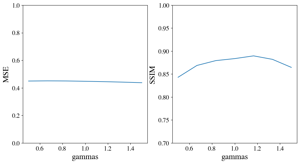
- Results : for this particular image, we checked that using the luminance ($\gamma \approx 1$) is the correct choice. The outcome is that gamma correction may improve coding, but only slightly. In the figure below, we plot as a function of gamma the final energy of the error and the perceptually relevant measure of structural simailarity :
-
This may not be the case for other types of images which would justify an image-by-image local gain control.
-
more information on sparse coding is exposed in the following book chapter (see also https://laurentperrinet.github.io/publication/perrinet-15-bicv ):
@inbook{Perrinet15bicv,
    title = {Sparse models},
    author = {Perrinet, Laurent U.},
    booktitle = {Biologically-inspired Computer Vision},
    chapter = {13},
    editor = {Keil, Matthias and Crist\'{o}bal, Gabriel and Perrinet, Laurent U.},
    publisher = {Wiley, New-York},
    year = {2015}
}
setting up the sparse coding framework
In [1]:
import numpy as np
from SparseEdges import SparseEdges
mp = SparseEdges('https://raw.githubusercontent.com/bicv/SparseEdges/master/default_param.py')
if not mp.pe.do_whitening: print('\!/ Wrong parameters... \!/')

# where should we store the data + figures generated by this notebook
import os
mp.pe.do_mask = True
# mp.pe.use_cache = False

mp.pe.N_X, mp.pe.N_Y = 256, 256

mp.pe.N = 1024
#mp.pe.N = 2048
#mp.pe.N = 64
# name = f'/tmp/2019-11-13-B_progressive'
mp.pe.matpath, mp.pe.figpath = '../files/2015-05-22-a-hitchhiker-guide-to-matching-pursuit', '../files/2015-05-22-a-hitchhiker-guide-to-matching-pursuit'
mp.pe.MP_alpha = 1.
mp.pe.MP_alpha = .8

mp.pe.mask_exponent = 6.
mp = SparseEdges(mp.pe)
mp.init()
print('mp.pe.N_X, mp.pe.N_Y', mp.pe.N_X, mp.pe.N_Y)
# defining input image (get it @ https://www.flickr.com/photos/doug88888/6370387703)
# https://images2.minutemediacdn.com/image/upload/c_crop,h_1286,w_2288,x_0,y_12/v1553818270/shape/mentalfloss/70991-istock-638419754.jpg

print('Default parameters: ', mp.pe)
The useful imports for a nice notebook:
In [2]:
import matplotlib
fontsize = 15
matplotlib.rcParams['figure.max_open_warning'] = 400
matplotlib.rcParams.update({'text.usetex': False,
                            'axes.labelsize':19,
                            'xtick.labelsize':fontsize,
                            'ytick.labelsize':fontsize,
                            'legend.fontsize':fontsize,
                           })
import matplotlib.pyplot as plt

%matplotlib inline
%config InlineBackend.figure_format='retina'
import matplotlib.pyplot as plt

import numpy as np
np.set_printoptions(precision=4)#, suppress=True)

fig_width = 14
In [3]:
print('Range of spatial frequencies: ', mp.sf_0)
In [4]:
print('Range of angles (in degrees): ', mp.theta*180./np.pi)
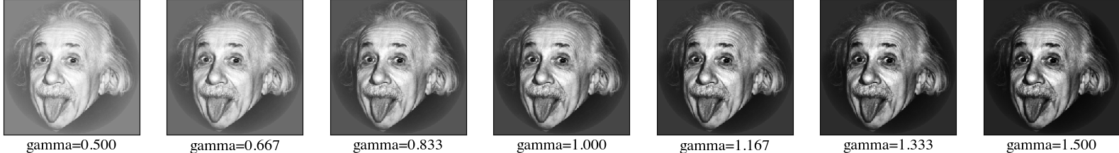
coding one image with different gammas
In [5]:
from SLIP import imread
SHOW = True
In [6]:
def normalize(image, do_full=True, verbose=SHOW):
    if do_full: # normalizes in the full range between 0 and 1
        if verbose: print('in norm', image.mean(), image.min(), image.max())
        image -= image.min()
        if verbose: print('decenter', image.mean(), image.min(), image.max())
        image /= image.max()
        if verbose: print('max out', image.mean(), image.min(), image.max())
    else:# normalizes such that the mean is .5 and the extremum is 0 or 1
        if verbose: print('in norm', image.mean(), image.min(), image.max())
        image -= image.mean()
        if verbose: print('decenter', image.mean(), image.min(), image.max())
        image /= np.abs(image).max()
        if verbose: print('max out', image.mean(), image.min(), image.max())
        image *= .5
        if verbose: print('max out', image.mean(), image.min(), image.max())
        image += .5
        if verbose: print('recenter', image.mean(), image.min(), image.max())
    return image

def preprocess(image, gamma=1, verbose=SHOW):
    if verbose: print('preproc', image.mean(), image.min(), image.max())
    image = normalize(image, do_full=True, verbose=verbose)
    if verbose: print('norm', image.mean(), image.min(), image.max())
    image = image**gamma
    if verbose: print('out', image.mean(), image.min(), image.max())
    return image

def deprocess(white, gamma=1, verbose=SHOW):

    image = mp.dewhitening(white)
    if image.max() > image.min(): image = normalize(image, do_full=True)
    image = image**(1/gamma)
    if image.max() > image.min(): image = normalize(image, do_full=True)

    return image
In [7]:
from SLIP import imread
url = 'https://upload.wikimedia.org/wikipedia/commons/d/d7/Meisje_met_de_parel.jpg'
url = 'https://farm7.staticflickr.com/6058/6370387703_5e718ea681_q_d.jpg'
url = 'https://upload.wikimedia.org/wikipedia/en/1/1e/Frida_Kahlo_%28self_portrait%29.jpg'
url = 'http://1.bp.blogspot.com/-EIqqVOCuIcE/T5HfIXEk05I/AAAAAAAAARk/NzQrgFJ5itI/s1600/einstein.jpg'
image = imread(url)
print('image shape=', image.shape)
In [8]:
# TODO make it square
In [9]:
#image = mp.imread(os.path.join(mp.pe.matpath, '6370387703_5e718ea681_q_d.jpg'))
from skimage.transform import resize
image = resize(image, (mp.pe.N_X, mp.pe.N_Y))
print('image shape=', mp.pe.N_X, mp.pe.N_Y, image.shape)
if SHOW: print('in', image.mean(), image.min(), image.max())
image = mp.preprocess(image)
if SHOW: print('before process', image.mean(), image.min(), image.max())
image = preprocess(image, gamma=1.)
if SHOW: print('before mask', image.mean(), image.min(), image.max())
#if mp.pe.do_mask: image = (image-image.mean())*mp.mask + image.mean()
if mp.pe.do_mask:
    im_med = np.median(image)
    image = (image-im_med)*mp.mask + im_med
if SHOW: print('after mask', image.mean(), image.min(), image.max())
image_original = image.copy()
In [10]:
gammas = np.linspace(.5, 1.5, 7)
print('gammas =', gammas)
In [11]:
fig, axs = plt.subplots(1, len(gammas), figsize=(21, 5))
for gamma, ax in zip(gammas, axs):
    image = image_original.copy()
    image = preprocess(image, gamma=gamma, verbose=False)
    ax.imshow(image, vmin=0, vmax=1, cmap=plt.gray())
    ax.set_xticks([])
    ax.set_yticks([])
    ax.set_xlabel(f'gamma={gamma:.3f}', fontsize=16)
import os
fig.savefig(os.path.join(mp.pe.figpath, 'gamma.png'), dpi=100, bbox_inches='tight', pad_inches=0)

In [12]:
fig, axs = plt.subplots(1, len(gammas), figsize=(21, 5))
for gamma, ax in zip(gammas, axs):
    image = image_original.copy()
    image = preprocess(image, gamma=gamma, verbose=False)
    ax.hist(image.ravel(), bins=np.linspace(0, 1, 50), alpha=.3, label=gamma, density=True)

    ax.set_xlim([0, 1])
    #ax.set_xlabel('gammas')
    ax.set_xlabel(f'gamma={gamma:.3f}', fontsize=16)
    ax.set_yscale('log')
axs[0].set_ylabel('intensity', fontsize=16)
#_ = plt.legend()
Out[12]:

Processing one image with different values of gamma:
In [13]:
for gamma in gammas:
    name = f'MP_gamma_{gamma}'
    print('processing ', name)
    matname = os.path.join(mp.pe.matpath, name + '.npy')
    image = image_original.copy()
    image = preprocess(image, gamma=gamma, verbose=False)

    white = mp.whitening(image)

    try:
        edges = np.load(matname)
    except:
        edges, C_res = mp.run_mp(white, verbose=True)
        np.save(matname, edges)

    i_Ns = np.arange(0, mp.pe.N, 16)
    matname_MSE = os.path.join(mp.pe.matpath, name + '_MSE.npy')
    matname_SSIM = os.path.join(mp.pe.matpath, name + '_SSIM.npy')
    try:
        MSE = np.load(matname_MSE)
        SSIM = np.load(matname_SSIM)
    except:
        image_original_crop = image_original[mp.pe.N_X//4:(mp.pe.N_X*3)//4, mp.pe.N_Y//4:(mp.pe.N_Y*3)//4]
        MSE = np.zeros(len(i_Ns))
        # https://scikit-image.org/docs/dev/auto_examples/transform/plot_ssim.html
        from skimage.metrics import structural_similarity as ssim
        opts_ssim = dict(multichannel=False, gaussian_weights=True, sigma=1.5, use_sample_covariance=False)
        SSIM = np.zeros(len(i_Ns))
        for ii_N, i_N in enumerate(i_Ns):
            white_rec = mp.reconstruct(edges[:, :i_N])
            MSE[ii_N] =  ((white-white_rec)**2).mean()
            image_rec = deprocess(white_rec, gamma=gamma)
            image_rec_crop = image_rec[mp.pe.N_X//4:(mp.pe.N_X*3)//4, mp.pe.N_Y//4:(mp.pe.N_Y*3)//4]
            SSIM[ii_N] =  ssim(image_original_crop, image_rec_crop,
                              data_range=image_rec_crop.max() - image_rec_crop.min())
        np.save(matname_MSE, MSE)
        np.save(matname_SSIM, SSIM)
In [14]:
gamma = 1.
name = f'MP_gamma_{gamma}'
matname = os.path.join(mp.pe.matpath, name + '.npy')
edges = np.load(matname)
In [15]:
white_rec = mp.reconstruct(edges)
image_rec = deprocess(white_rec, gamma=gamma, verbose=False)

fig_width_pt = 318.670  # Get this from LaTeX using \showthe\columnwidth
inches_per_pt = 1.0/72.27               # Convert pt to inches
fig_width = fig_width_pt*inches_per_pt  # width in inches
mp.pe.figsize_edges = .382 * fig_width  # useful for papers
mp.pe.figsize_edges = 9 # useful in notebooks
mp.pe.line_width = 1.
mp.pe.scale = 1.
fig, a = mp.show_edges(edges, image=2*image_rec-1, show_phase=True, show_mask=True)
#mp.savefig(fig, name + '_rec')

A nice property of Matching Pursuit is that one can reconstruct the image from the edges:
In [16]:
white_rec = mp.reconstruct(edges)
print('remaining energy  = ', ((white-white_rec)**2).sum()/(white**2).sum()*100, '%')
The whitened reconstructed image looks like:
In [17]:
image_rec = deprocess(white_rec, gamma=gamma, verbose=False)
fig, a = mp.show_edges(edges, image=image_rec);

let's check how this varies with gamma:
In [18]:
MSE_0 = (white**2).sum()

plt.figure(figsize=(12,6))
plt.subplot(111)
for gamma in gammas:
    name = f'MP_gamma_{gamma}'
    matname_MSE = os.path.join(mp.pe.matpath, name + '_MSE.npy')
    MSE = np.load(matname_MSE)
    plt.plot(i_Ns, MSE/MSE[0], 'o', label=f'MP_gamma_{gamma:.3f}', alpha=.2)
plt.xlim([0, mp.pe.N])
plt.ylim([0, 1])
plt.xlabel('# atoms')
plt.ylabel('MSE')
_ = plt.legend()

In [19]:
plt.figure(figsize=(12,6))
plt.subplot(111)
for gamma in gammas:
    name = f'MP_gamma_{gamma}'
    matname_SSIM = os.path.join(mp.pe.matpath, name + '_SSIM.npy')
    SSIM = np.load(matname_SSIM)
    plt.plot(i_Ns, SSIM, 'o', label=f'MP_gamma_{gamma:.3f}', alpha=.2)
plt.xlim([0, mp.pe.N])
plt.ylim([0, 1])
plt.xlabel('# atoms')
plt.ylabel('SSIM')
_ = plt.legend()

In [23]:
MSE_0 = (white**2).sum()

fig, axs = plt.subplots(1, 2, figsize=(12,6))
MSEs, SSIMs = [], []
for gamma in gammas:
    name = f'MP_gamma_{gamma}'
    matname_MSE = os.path.join(mp.pe.matpath, name + '_MSE.npy')
    MSE = np.load(matname_MSE)
    MSEs.append(MSE[-1]/MSE[0])
    matname_SSIM = os.path.join(mp.pe.matpath, name + '_SSIM.npy')
    SSIM = np.load(matname_SSIM)
    SSIMs.append(SSIM[-1])

axs[0].plot(gammas, np.sqrt(MSEs))
axs[0].set_ylim([0, 1])
axs[0].set_xlabel('gammas')
axs[0].set_ylabel('MSE')
axs[1].plot(gammas, SSIMs)
axs[1].set_ylim([0.7, 1])
axs[1].set_xlabel('gammas')
axs[1].set_ylabel('SSIM')
fig.savefig(os.path.join(mp.pe.figpath, 'gamma_results.png'), dpi=100, bbox_inches='tight', pad_inches=0.1)

some book keeping for the notebook
In [21]:
#%ls -l ../files/2015-05-22-a-hitchhiker-guide-to-matching-pursuit/
#%rm ../files/2015-05-22-a-hitchhiker-guide-to-matching-pursuit/MP_gamma*
#%rm ../files/2015-05-22-a-hitchhiker-guide-to-matching-pursuit/MP_gamma*MSE*
#%rm ../files/2015-05-22-a-hitchhiker-guide-to-matching-pursuit/MP_gamma*SSIM*
#%rm ../files/2015-05-22-a-hitchhiker-guide-to-matching-pursuit/MP_gamma*npy
In [22]:
%load_ext watermark
%watermark -i -h -m -v -p numpy,SLIP,LogGabor,SparseEdges,matplotlib  -r -g -b