Recruiting different population ratios in V1 using MotionClouds' orientation components
InViBe's Journal Club - https://intranet.int.univ-amu.fr/fr/invibe/journalclub
- (sep 26th) Laurent : introduction https://laurentperrinet.github.io/sciblog/files/2016-09-26_Perrinet16journalClub/2016-09-26_Perrinet16journalClub.slides.html
- (oct 3rd) Frédo : Origin and Function of Tuning Diversity in Macaque Visual Cortex by Robbe L.T. Goris, Eero P. Simoncelli, J. Anthony Movshon - http://www.sciencedirect.com/science/article/pii/S0896627315008752
- (oct 10th) : free slot (IRM?)
- (oct 17th) : Ivo
- (oct 24th and 31st) : break
- (nov 7th) Christopher : psychophysics
See https://laurentperrinet.github.io/sciblog/posts/2014-11-10_orientation.html
Re-compile this presentation using https://laurentperrinet.github.io/sciblog/files/2016-09-26_Perrinet16journalClub/2016-09-26_Perrinet16journalClub.ipynb
manipulating the bandwidth in MotionClouds
import numpy as np
import MotionClouds as mc
fx, fy, ft = mc.get_grids(mc.N_X, mc.N_Y, mc.N_frame)
name = 'balaV1'
N_X = fx.shape[0]
width = 29.7*256/1050
sf_0 = 4.*width/N_X
B_V = 2.5 # BW temporal frequency (speed plane thickness)
B_sf = sf_0 # BW spatial frequency
theta = 0.0 # Central orientation
B_theta_low, B_theta_high = np.pi/32, 2*np.pi
B_V = 0.5
seed=12234565
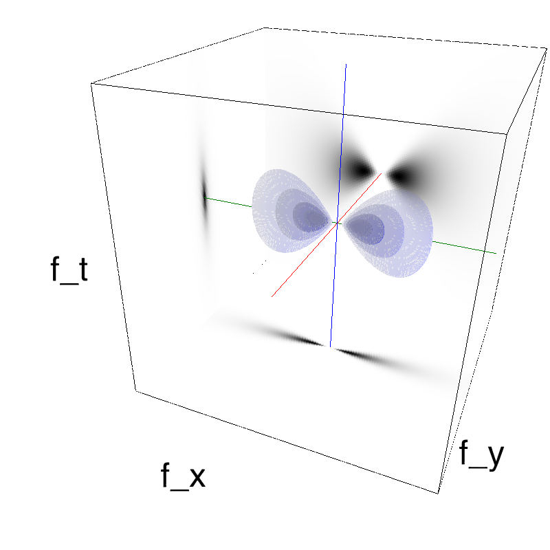
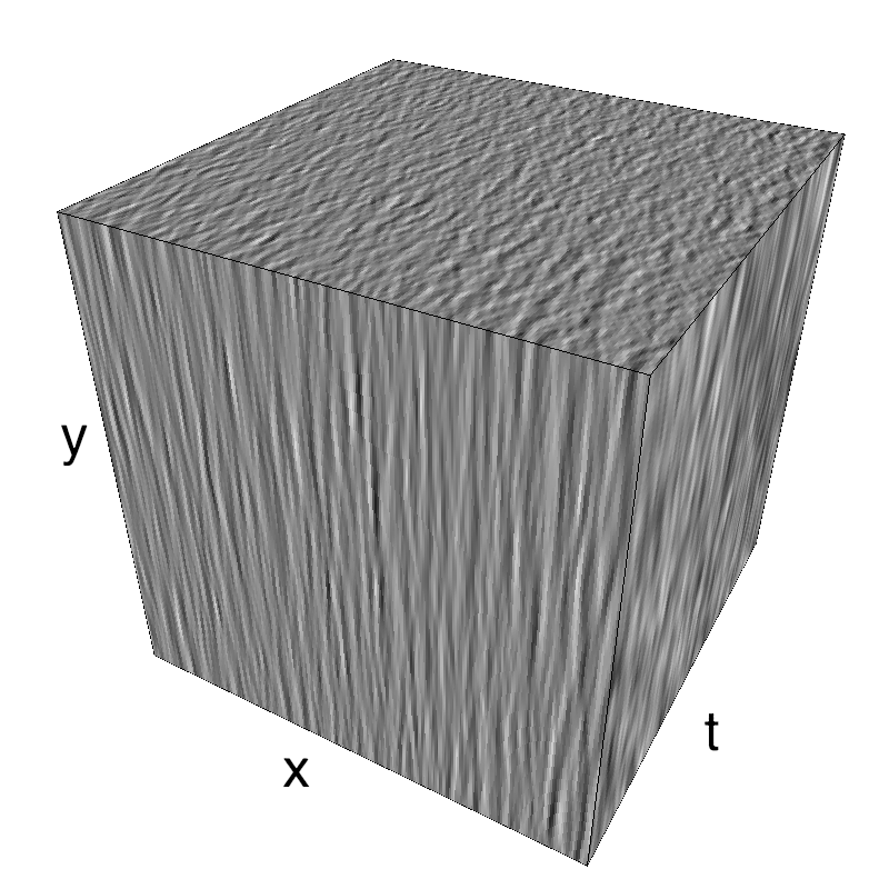
mc1 = mc.envelope_gabor(fx, fy, ft, V_X=0., V_Y=0., B_V=B_V, sf_0=sf_0, B_sf=B_sf, theta=theta, B_theta=B_theta_low)
In [2]:
import numpy as np
import MotionClouds as mc
mc.figpath = figpath
fx, fy, ft = mc.get_grids(mc.N_X, mc.N_Y, mc.N_frame)

name = 'balaV1'

N_X = fx.shape[0]
width = 29.7*256/1050
sf_0 = 4.*width/N_X
B_V = 2.5     # BW temporal frequency (speed plane thickness)
B_sf = sf_0   # BW spatial frequency
theta = 0.0   # Central orientation
B_theta_low, B_theta_high = np.pi/32, 2*np.pi
B_V = 0.5
seed=12234565

mc1 = mc.envelope_gabor(fx, fy, ft, V_X=0., V_Y=0., B_V=B_V, sf_0=sf_0, B_sf=B_sf, theta=theta, B_theta=B_theta_low)
name_ = name + '_1'
mc.figures(mc1, name_, seed=seed)
mc.in_show_video(name_, figpath=figpath)
 |
||
 |
||
In [3]:
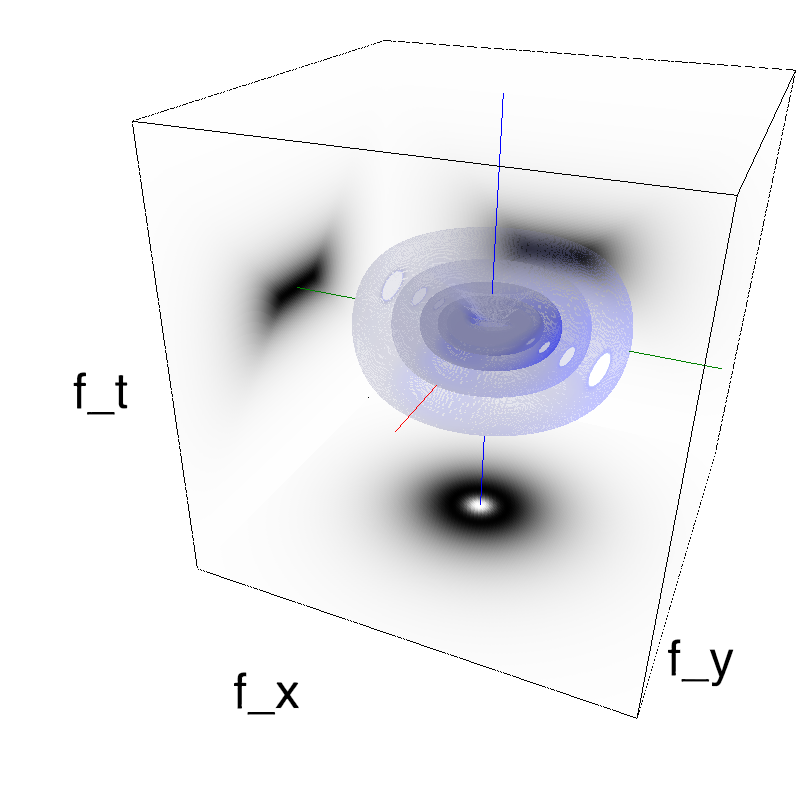
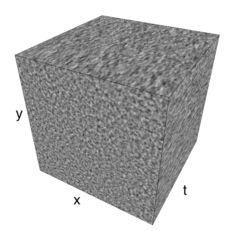
mc2 = mc.envelope_gabor(fx, fy, ft, V_X=0., V_Y=0., B_V=B_V, sf_0=sf_0, B_sf=B_sf, theta=theta, B_theta=B_theta_high)
name_ = name + '_2'
mc.figures(mc2, name_, seed=seed)
mc.in_show_video(name_, figpath=figpath)
 |
||
 |
||
Loi de Von Mises (loi normale circulaire) telle que $f(\theta+\pi) = f(\theta)$ définie par :
$$ f(\theta) \propto e^{\kappa{cos(2(\theta - m))}} $$Par analogie avec la déviation standard d'une loi Gaussienne, on définit $\kappa = \frac {1}{\sigma^{2}}$.
In [4]:
def envelope(th, theta, B_theta):
    if B_theta==np.inf:
        env = np.ones_like(th)
    elif B_theta==0:
        env = np.zeros_like(th)
        env[np.argmin(th < theta)] = 1.
    else:
        env = np.exp((np.cos(2*(th-theta))-1)/4/B_theta**2)
    return env/env.max()

N_theta = 12
bins = 180
th = np.linspace(0, np.pi, bins, endpoint=False)
fig, axs = plt.subplots(1, 2, figsize=(fig_width, fig_width/phi/2))
for i, B_theta_ in enumerate([np.pi/12, np.pi/4]):#[0, np.pi/64, np.pi/32, np.pi/16, np.pi/8, np.pi/4, np.pi/2, np.inf]:
    for theta, color in zip(np.linspace(0, np.pi, N_theta, endpoint=False),
                            [plt.cm.hsv(h) for h in np.linspace(0, 1, N_theta)]):
        axs[i].plot(th*180/np.pi, envelope(th, theta, B_theta_), alpha=.6, color=color, lw=3)
        axs[i].fill_between(th*180/np.pi, 0, envelope(th, theta, B_theta_), alpha=.1, color=color)
    axs[i].set_xlim([0, 180])
    axs[i].set_ylim([0, 1.1])
    axs[i].set_xticks(np.linspace(0, 180, 5, endpoint=True) )#to specify number of tick…
for ax in axs:
    for item in ([ax.title, ax.xaxis.label, ax.yaxis.label] +
                 ax.get_xticklabels() + ax.get_yticklabels()):
        item.set_fontsize(fontsize)

In [5]:
fx, fy, ft = mc.get_grids(mc.N_X, mc.N_Y, 1)


N_theta = 6
bw_values = np.pi*np.logspace(-2, -5, N_theta, base=2)


fig, axs = plt.subplots(1, N_theta, figsize=(fig_width, fig_width/N_theta))
for i_ax, B_theta in enumerate(bw_values):
    mc_i = mc.envelope_gabor(fx, fy, ft, V_X=0., V_Y=0.,
                                         theta=np.pi/2, B_theta=B_theta)
    im = mc.random_cloud(mc_i)

    axs[i_ax].imshow(im[:, :, 0], cmap=plt.gray())
    axs[i_ax].text(5, 29, r'$B_\theta=%.1f$°' % (B_theta*180/np.pi), color='white', fontsize=32)
    axs[i_ax].set_xticks([])
    axs[i_ax].set_yticks([])
plt.tight_layout()
fig.subplots_adjust(hspace = .0, wspace = .0, left=0.0, bottom=0., right=1., top=1.)

exploring differentsP bandwidths by smoothly varying $B_\theta$
In [6]:
name = 'smooth'
theta_phi = np.pi * (3 - np.sqrt(5)) # https://en.wikipedia.org/wiki/Golden_angle
if mc.check_if_anim_exist(name):
    fx, fy, ft = mc.get_grids(mc.N_X, mc.N_Y, mc.N_frame//2)
    smooth = (ft - ft.min())/(ft.max() - ft.min()) # smoothly progress from 0. to 1.
    seed = 123456

    B_theta_ = B_theta_high*2.**-np.arange(5)
    B_theta_ = np.hstack((B_theta_, B_theta_[1:-1][::-1]))
    print('Smoothly changing B_theta along', B_theta_, '... and so on...')

    im = np.empty(shape=(mc.N_X, mc.N_Y, 0))
    N = len(B_theta_)
    im =  np.empty(shape=(mc.N_X, mc.N_Y, 0))

    for i_theta, B_theta in enumerate(B_theta_):
        im_old = mc.random_cloud(mc.envelope_gabor(fx, fy, ft, theta=theta_phi, B_theta=B_theta, V_X=0), seed=seed)
        im_new = mc.random_cloud(mc.envelope_gabor(fx, fy, ft, theta=theta_phi, B_theta=B_theta_[(i_theta+1) % N], V_X=0), seed=seed)
        im = np.concatenate((im, (1.-smooth)*im_old+smooth*im_new), axis=-1)

    mc.anim_save(mc.rectif(im), os.path.join(mc.figpath, name))
#mc.in_show_video(name, figpath=figpath)
show_video(os.path.join(mc.figpath, name), height=.8*height, width=.8*height)
Out[6]:
The problem of detecting orientations : OB V1
- check out https://github.com/laurentperrinet/OBV1
In [7]:
show_image('https://raw.githubusercontent.com/laurentperrinet/OBV1/master/figs/Ben_Kenobi.png', height=height*.8)
Out[7]:
In [8]:
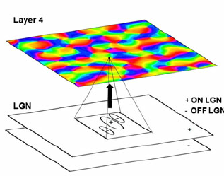
show_image('https://raw.githubusercontent.com/laurentperrinet/OBV1/master/figs/Fig-1-a-Model-Schematic-The-model-consists-of-the-three-major-subsystems-retina.png', height=.4*height)
Out[8]:
In [9]:
show_image('https://github.com/laurentperrinet/OBV1/raw/master/figs/pasturel_result.png', height=.4*height)
Out[9]:

In [10]:
show_image('https://raw.githubusercontent.com/laurentperrinet/OBV1/master/figs/nn3977-F1.jpg', height=height*.8)
Out[10]:
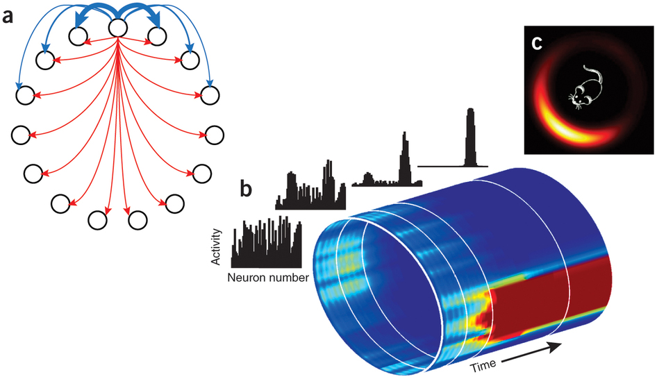
''The compass within'', Nathan W Schultheiss & A David Redish (Nature Neuroscience 18, 482–483 (2015) doi:10.1038/nn.3977 http://www.nature.com/neuro/journal/v18/n4/full/nn.3977.html)
In [11]:
show_image('https://raw.githubusercontent.com/laurentperrinet/OBV1/master/figs/future_model.png', height=height)
Out[11]:
In [12]:
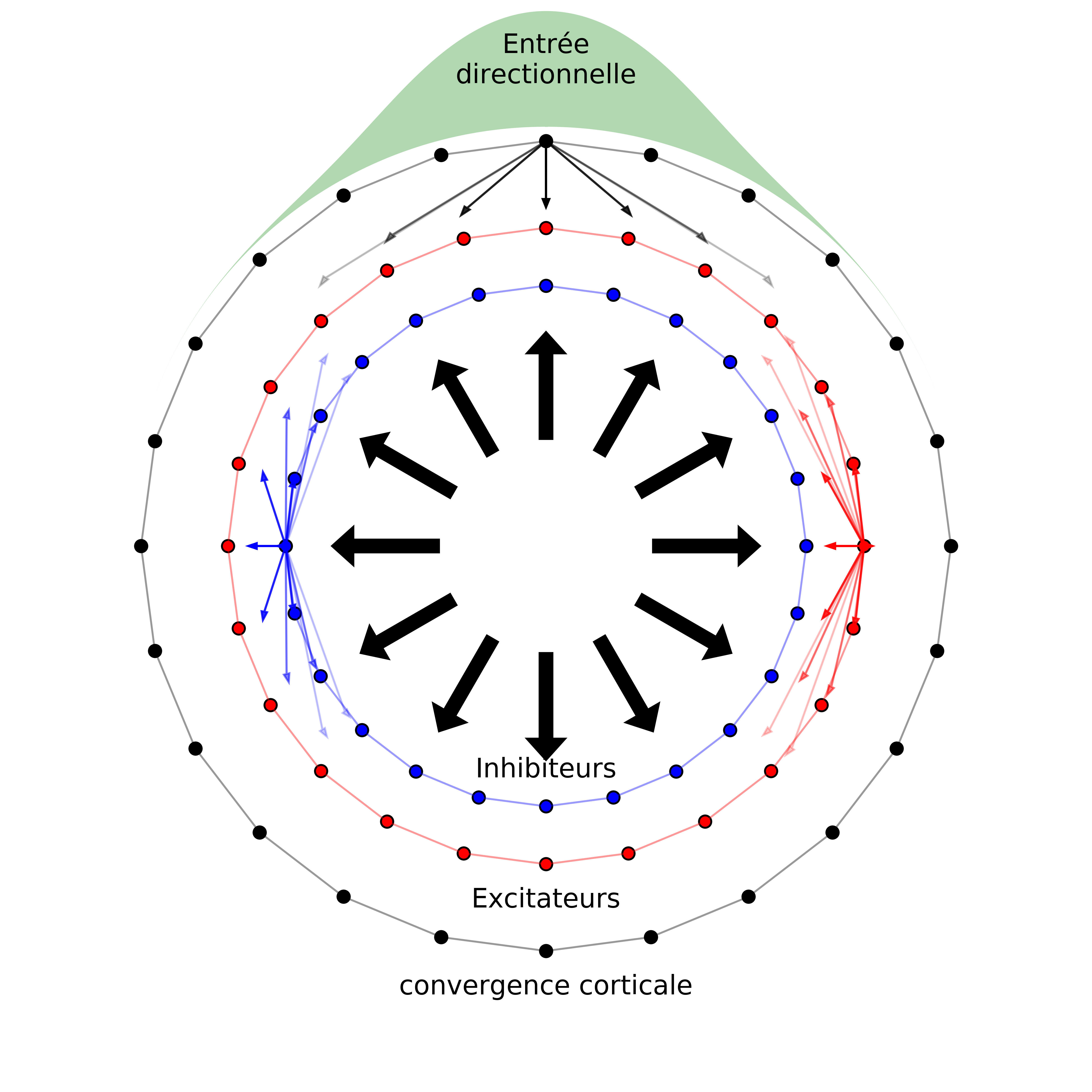
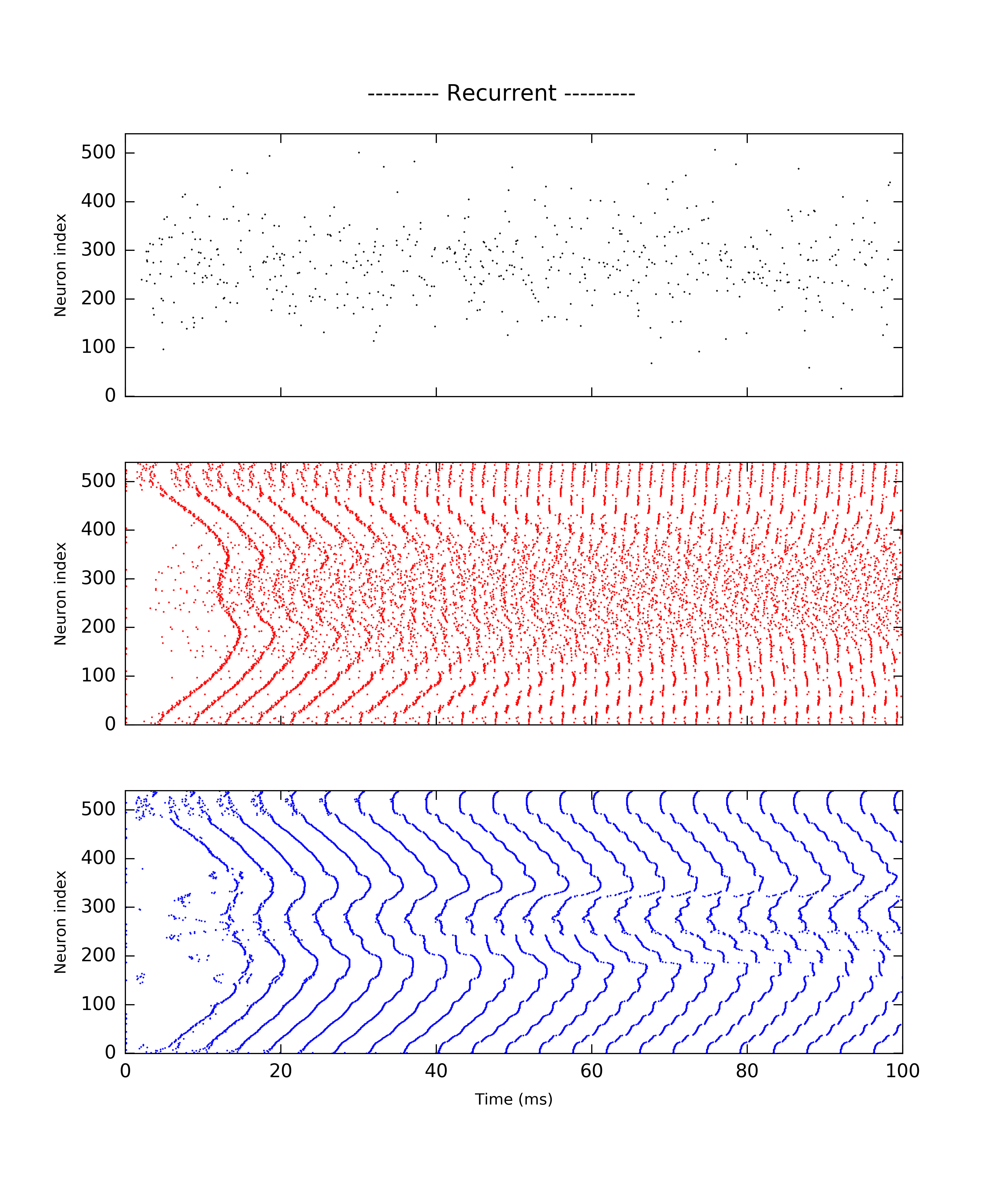
show_image('https://raw.githubusercontent.com/laurentperrinet/OBV1/master/figs/ringRecurrent.png', height=height)
Out[12]:
Recruiting different population ratios in V1 using MotionClouds' orientation components
questions and comments
- there may be links with models in texture discrimination (e.g. back pocket model from Landy), models with an association field, check-out TextureNet and al
- interaction with eye movements, e.g. Marisa Carrasco : sharpening of the tuning function at the instant of the saccade ( http://psych.nyu.edu/carrascolab/publications/LiBarbotCarrasco2016.pdf )
- effects of size of features (e.g. wrt to receptive field size)