HTML("""
<h1 class="title">Decoding of feature selectivity in neural activity</h1>
<h1>Concrete applications in visual data</h1>
<h2>Laurent U Perrinet, INT - Wahiba Taouali, INMED</h2>
<img src="figures/troislogos.png" width=61%/>
""")
Decoding of feature selectivity in neural activity
Concrete applications in visual data
Laurent U Perrinet, INT - Wahiba Taouali, INMED

- Course on Computational Neuroscience, Marseille, December 8th, 2015
Acknowledgements:
- PhD program: Anna Montagnini, Frédéric Chavane, Nadia Pittet, INT, Marseille
- Material: Peggy Series, Christopher Olah
- NeuroPhysiology: Giacomo Benvenuti, Frédéric Chavane, INT, Marseille
HTML("""
    <!-- <h2>Problem statement</h2> -->
    <video controls src="{1}" poster="{0}" width=100%/>
    """.format(figpath + 'scientists.jpg', figpath + 'ComplexDirSelCortCell250_title.webm')
)
Bayes : travelling back to the feature space
(see http://colah.github.io/posts/2015-09-Visual-Information/)
Image('figures/prob-1D-rain.png', height=height)

Image('figures/prob-1D-coat.png', height=height)

Image('figures/prob-2D-independent-rain.png', height=height)

Image('figures/prob-2D-dependant-rain-squish.png', height=height)

Image('figures/prob-2D-factored-rain-arrow.png', height=height)

Image('figures/prob-2D-factored1-clothing-B.png', height=height)

examples of Bayesian mechanism in perception
Image('figures/jov-2-6-6-fig002.jpeg', height=height)
# http://jov.arvojournals.org/article.aspx?articleid=2121565

Image('figures/dotsconvex.jpeg', height=height)

Image('figures/dotsconcave.jpeg', height=height)

Image('figures/hollow_mask.jpg', height=height)

summary
Image('figures/encoding_problem.png', height=height)

summary
Image('figures/decoding_problem.png', height=height)

Image('figures/neural_activity_1.png', height=height)

Image('figures/neural_activity_2.png', height=height)

Image('figures/neural_activity_3.png', height=height)

Image('figures/neural_activity_4.png', height=height)

Image('figures/neural_activity_5.png', height=height)

HTML("""
<h2>Optimal representation of sensory information </h2>
<table border="0" width=100%/>
<tr>
<td width=50%/><img src="{0}" width=75%/> </td>
<td width=50%/><img src="{1}" width=100%/> </td>
</tr>
</table>
<em>Mehrdad Jazayeri & J Anthony Movshon</em> (2007) Nature Neuroscience
""".format(figpath + 'Jazayeri07optimal_figure1.png', figpath + 'Jazayeri07optimal_figure2.png'))
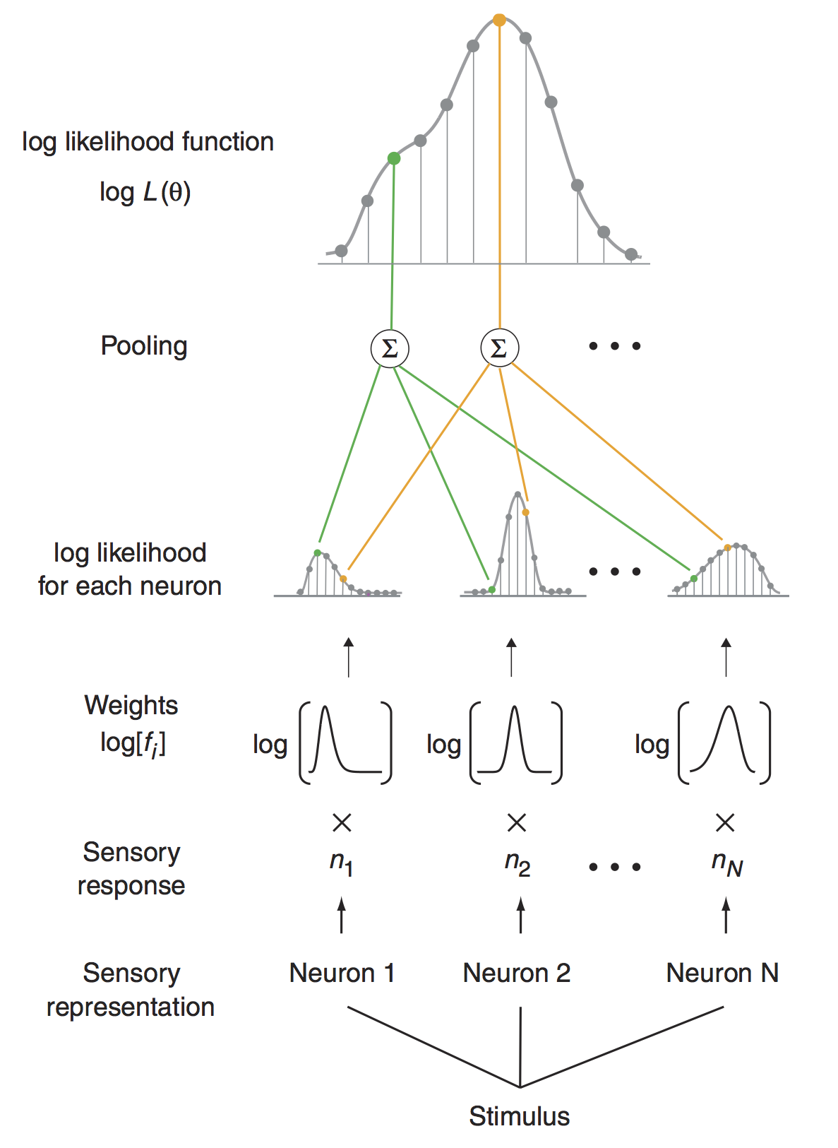
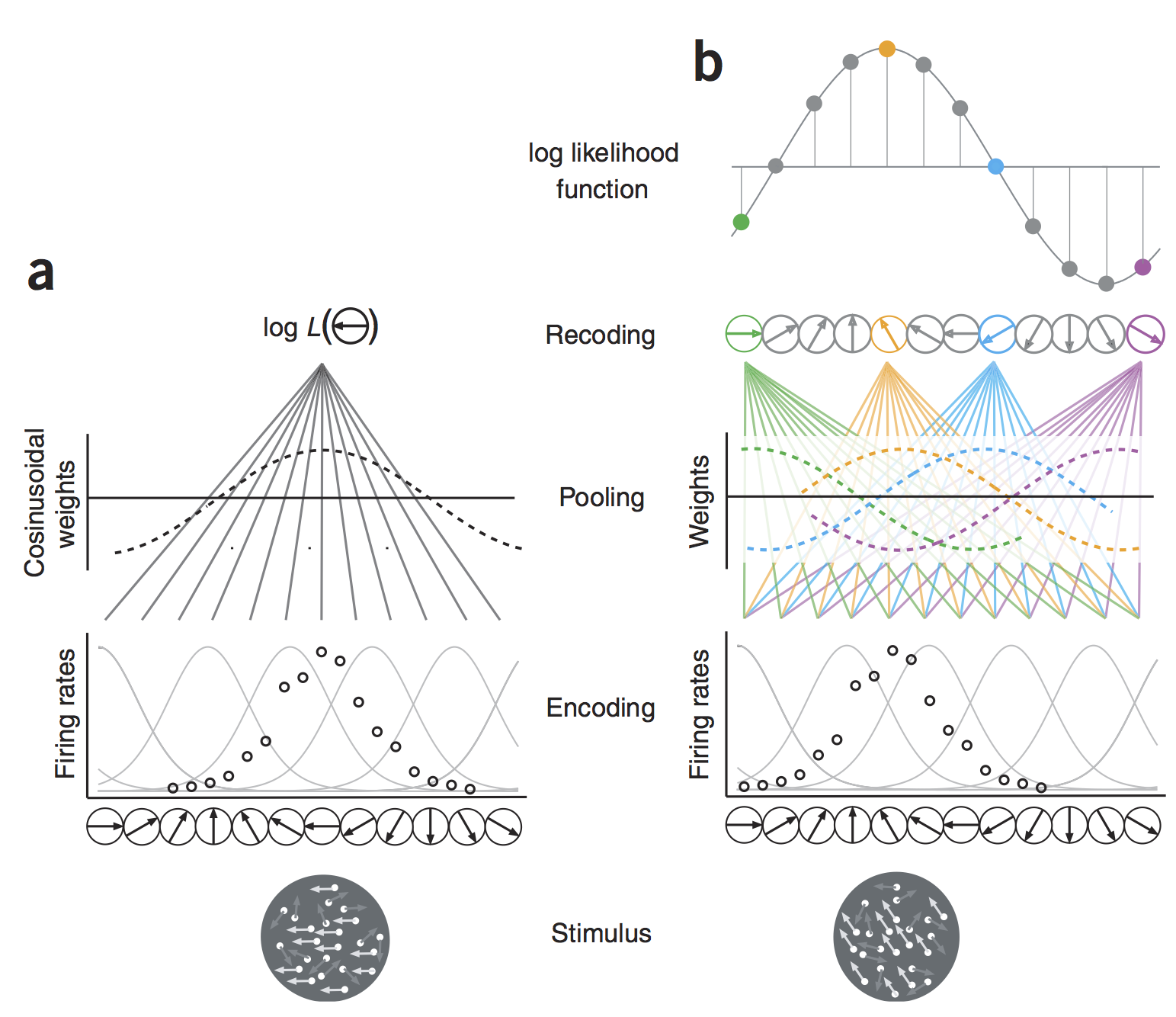
Optimal representation of sensory information
 |
 |
let's look at the proof
The definition of a tuning function that accounts for the modulation of the parameters of the variability model (mean, shape, scale, std) when we vary the stimili : f($\theta$)= mean(k|$\theta$) which gives : \begin{equation} P(k|{\theta}) = \frac{f({\theta}) ^{k}e^{-f({\theta})}}{k!} \end{equation}
The pooling of the population information : by the independence hypothesis, the probability of having a population response Y = [k{1}, k{2}.. k_{N}] (vector of N cells responses):
- Bayes' rule.
Maximum likelihood decoding.
The decoding algorithm consists of maximizing the posterior probability $P({\theta}|Y)$ as a function of the estimated direction ${\theta}$, given a distribution hypothesis:
- The evidence term $P(Y)$ is a normalization term independent of ${\theta}$ $\to P(Y)$=cst
- There is no prior knowledge on ${\theta}$ (such that $ \forall \theta_1, \theta_2$, $P(\theta_1)$ = $P(\theta_2)$)
Thus, maximizing the posterior $P(\theta|Y)$ under the Poisson hypothesis is equivalent to maximizing the following likelihood function: \begin{equation} L(\theta) = P(Y|{\theta}) = \Pi ^N _{i=1} \frac{f_i({\theta}) ^{k_i}e^{-f_i({\theta})}}{k_i!} \end{equation}
In practice, It is often the log-likelihood function that is considered:
\begin{equation} LL(\theta) = log(P(Y|{\theta})) = \sum_{i=1}^N{k_i\log[f_{i}(\theta)]}-\sum_{i=1}^N{f_{i}(\theta)}- \sum_{i=1}^N \log[{k_i!}] \end{equation}In the end:
\begin{equation} LL(\theta) = \sum_{i=1}^N{k_i\log[f_{i}(\theta)]} - \log(Z) \end{equation}HTML("""
<h2>Poisson distribution as a model of variability </h2>
<table border="0" width=100%/>
<tr>
<td width=50%/><embed src="{0}" width=100% '> </td>
<td width=50%/><embed src="{1}" width=100% '> </td>
</tr>
</table>""".format(figpath+ 'CellRasterV1.png',figpath+ 'DirectionTuningV1.png'))
Image('figures/antigravity.png', height=height)

python in neuroscience
Image('figures/python-in-neuroscience.png', height=height)

Python in Neuroscience
    ● Scientific python tools : Numpy, Scipy

    ● Plotting tools : Matplotlib

    ● Python interfaces to most major neuroscience software tools

        ● e.g. PyNN, PyNEURON, PyNEST, Brian

        ● Neurotools
Python vs. Matlab
Image('figures/python-matlab.png', height=height)

Ipython Notebook
    ● Interactive shell

    ● enhanced introspection,

    ● code highlighting

● tab completionHTML("""
<h1 class="title">Decoding of feature selectivity in neural activity</h1>
<h1>Concrete applications in visual data</h1>
<h2>Laurent U Perrinet, INT - Wahiba Taouali, INMED</h2>
<img src="figures/troislogos.png" width=61%/>
""")
Decoding of feature selectivity in neural activity
Concrete applications in visual data
Laurent U Perrinet, INT - Wahiba Taouali, INMED
Acknowledgements:
- PhD program: Anna Montagnini, Frédéric Chavane, Nadia Pittet, INT, Marseille
- Material: Peggy Series, Christopher Olah
- NeuroPhysiology: Giacomo Benvenuti, Frédéric Chavane, INT, Marseille