In [11]:
HTML("""
<h1 class="title">Decoding of feature selectivity in neural activity</h1>
<h1>Concrete applications in visual data</h1>
<h2>Wahiba Taouali, INMED - Laurent U Perrinet, INT</h2>
 <img src="{0}" height=61%/>
 """.format(figpath + 'troislogos.png'))
Out[11]:
Decoding of feature selectivity in neural activity
Concrete applications in visual data
Wahiba Taouali, INMED - Laurent U Perrinet, INT

Acknowledgements:
- PhD program: Anna Montagnini, Frédéric Chavane, Nadia Pittet, INT, Marseille
- Material: Peggy Series, Christopher Olah
- NeuroPhysiology: Giacomo Benvenuti, Frédéric Chavane, INT, Marseille
In [12]:
HTML("""
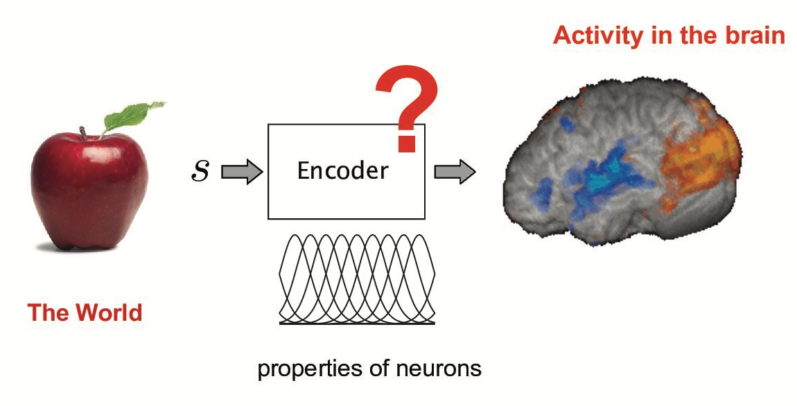
<h2>Reverse engineering : from encoding to decoding</h2>
<img src="{0}" width=100%/>
""".format(figpath + 'encoding_problem.png'))
Out[12]:
Reverse engineering : from encoding to decoding
In [13]:
HTML("""
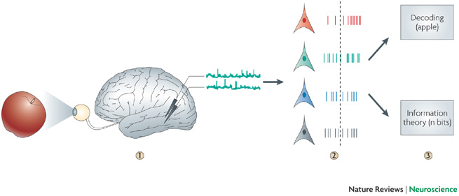
<h2>Reverse engineering : from encoding to decoding</h2>
<img src="{0}" width=100%/>
""".format(figpath + 'decoding.jpg'))
Out[13]:
Reverse engineering : from encoding to decoding
Neural data analysis
In [14]:
HTML("""
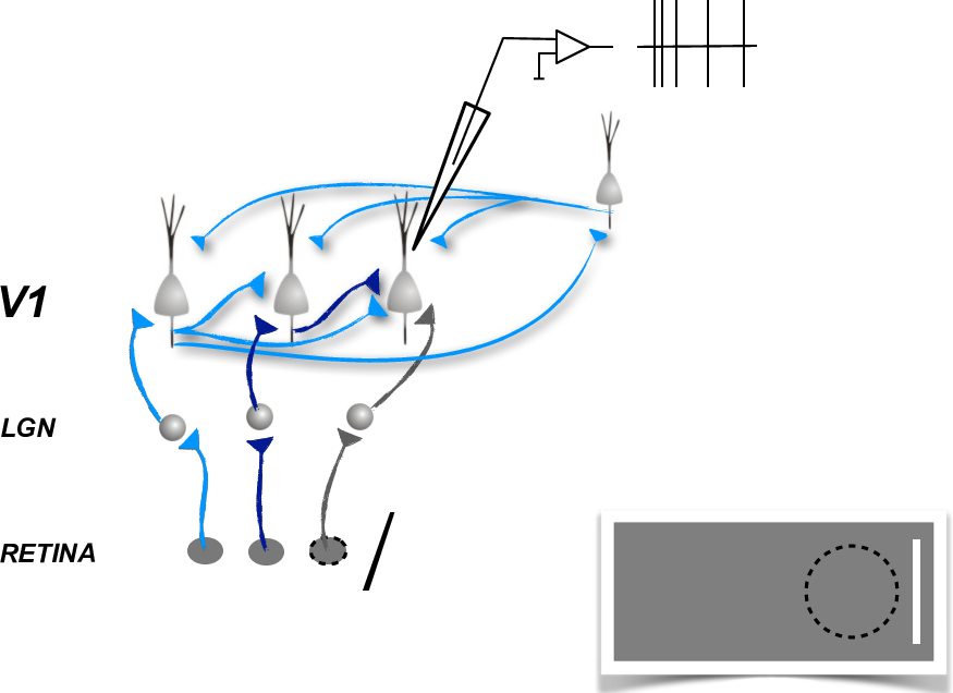
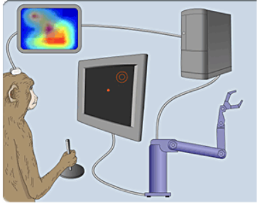
<h2>Experimental setup</h2>
<center><img src="{0}" height=60%/>
""".format(figpath + 'ExperimentalSetup_1.png'))
Out[14]:
Experimental setup

In [15]:
HTML("""
 <h2>Experimental setup</h2>
 <center><img src="{0}" height=60%/>
 """.format(figpath + 'ExperimentalSetup_2.png'))
Out[15]:
Experimental setup
In [16]:
HTML("""
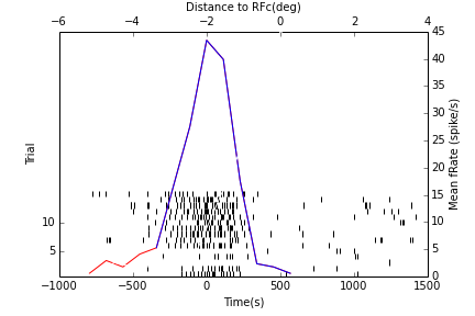
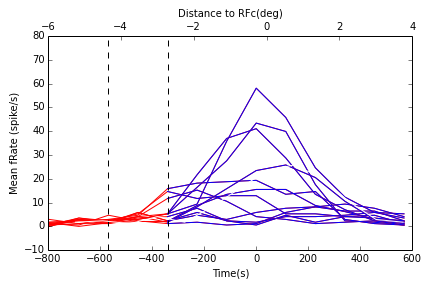
<h2>Describing neurons's activity </h2>
<table border="0" width=100%/>
<tr>
<td width=50%/><img src="{0}" width=100%/> </td>
<td width=50%/><img src="{1}" width=100%/> </td>
</tr>
</table>
""".format(figpath+ 'cell_response_c.png',figpath+ 'cell_response_all.png')
)
Out[16]:
Describing neurons's activity
 |
 |
In [17]:
HTML("""
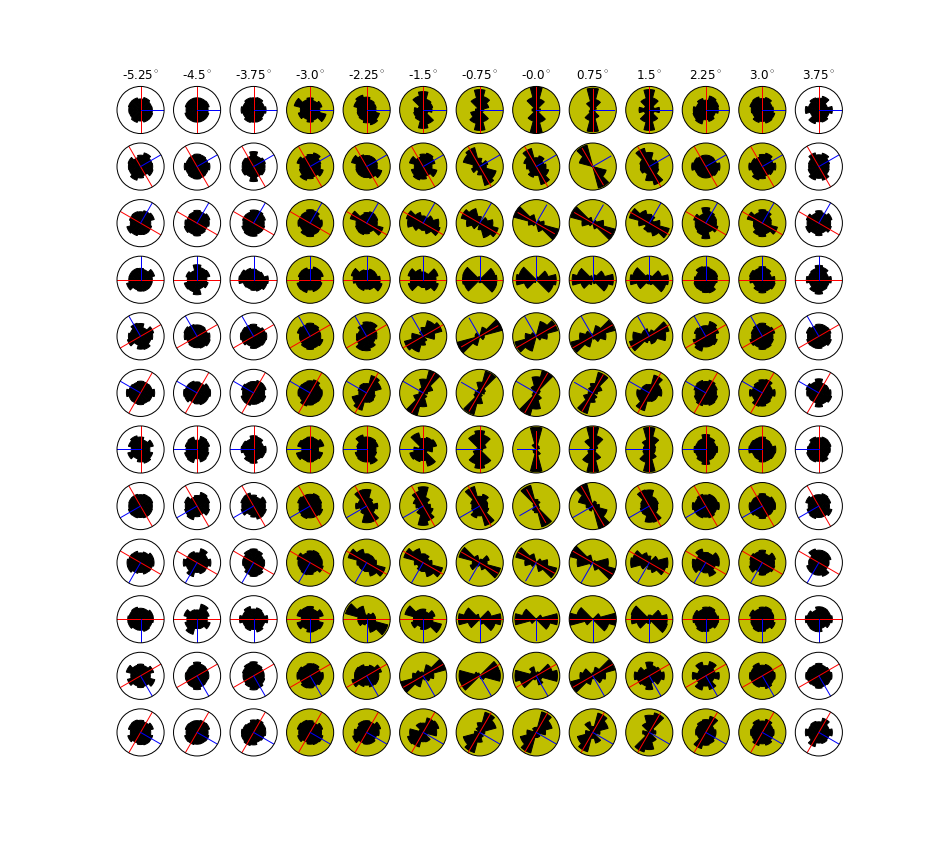
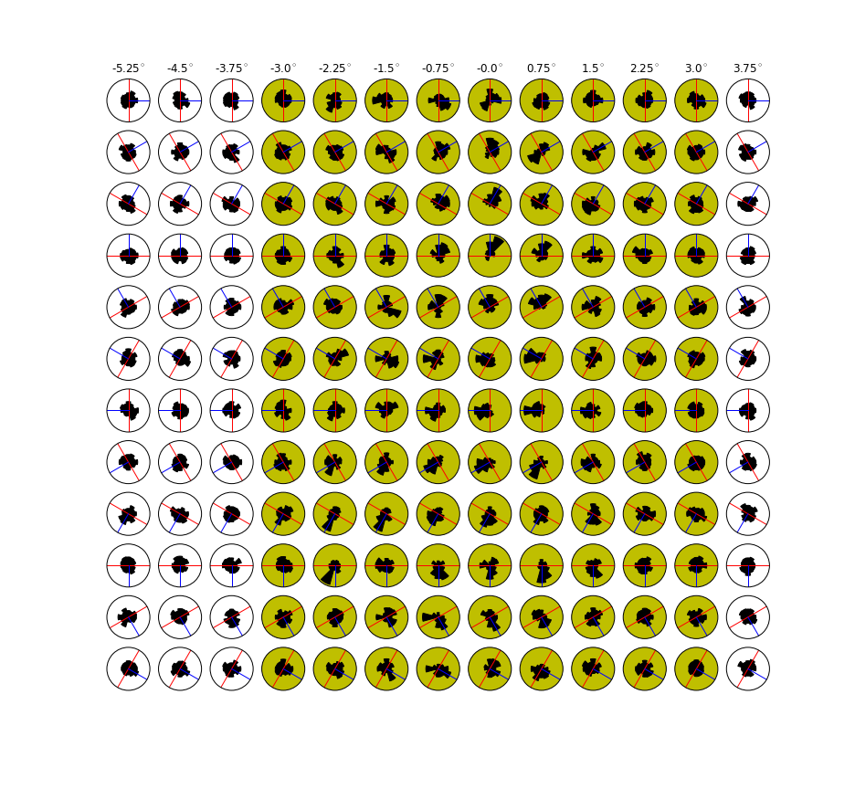
<h2>Tuning and Population statistics in RFc</h2>
<table border="0" width=100%/>
<tr>
<td width=30%/><embed src="{0}" width=100% > </td>
<td width=30%/><embed src="{1}" width=100% ></td>
<td width=30%/><embed src="{2}" width=100% > </td>
</tr>
</table>""".format(figpath+ 'TuningV1_population_average_1.png',figpath+ 'TuningV1_preferred_direction.png',figpath+ 'TuningV1_preferred_orientation_.png'))
Out[17]:
In [18]:
HTML("""
 <h2>Population dynamic decoding : orientation</h2>
  <center><img src="{0}" width=100%/>
 """.format(figpath+ 'decoding_orientation.png'))
Out[18]:
Population dynamic decoding : orientation
In [19]:
HTML("""
 <h2>Population dynamic decoding : direction</h2>
 <center><img src="{0}" width=100%/>
 """.format(figpath+ 'decoding_direction.png'))
Out[19]:
Population dynamic decoding : direction
In [20]:
HTML("""
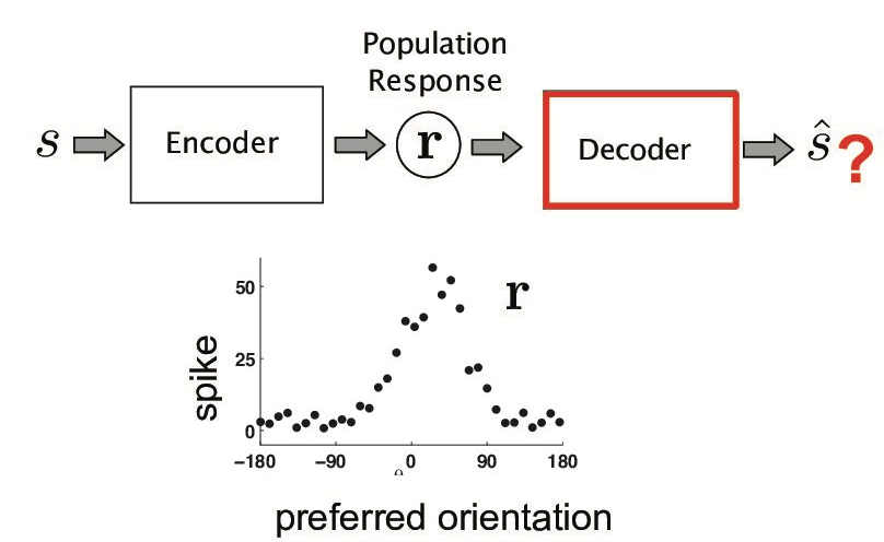
<h2>How to construct a decoder??</h2>
<img src="{0}" width=100%/>
""".format(figpath + 'decoding_problem.png'))
Out[20]:
How to construct a decoder??
Decoding approach
In [21]:
HTML("""
 <h2>Poisson distribution as a model of variability </h2>
 <table border="0" width=100%/>
    <tr>
    <td width=50%/><embed src="{0}" width=100% '> </td>
    <td width=50%/><embed src="{1}" width=100%  '> </td>
    </tr>
    </table>""".format(figpath+ 'CellRasterV1.png',figpath+ 'DirectionTuningV1.png'))
Out[21]:
In [22]:
HTML("""
 <h2>Von Mises as a model of Tuning </h2>
 <center>
    <table border="0" width=100%/>
    <tr>
    <td width=50%/><embed src="{0}" width=100%'> </td>
    <td width=50%/><embed src="{1}" width=100%'> </td>
    </tr>
    </table>
 """.format(figpath+ '2D_tuning.png',figpath+ 'TuningV1.png')
    )
Out[22]:
In [23]:
HTML("""
 <h2>Dynamic Tuning </h2>
    <table border="0" width=100%/>
    <tr height=30%/><embed src="{0}" width=100%'></tr>
    <tr height=30%/><embed src="{1}" width=100%'></tr>
    <tr height=30%/><embed src="{2}" width=100%'></tr>
    </table>
 """.format(figpath+ 'dynamic_tuning.png',figpath+ 'dynamic_tuning_1.png',figpath+ 'dynamic_tuning_2.png')
    )
Out[23]:
In [24]:
HTML("""
 <h2>Evaluation of decoding</h2>Leave-One-Out Cross Validation
 <img src="{0}" width=80%/>
 """.format(figpath+ 'loo.png'))
Out[24]:
Evaluation of decoding
Leave-One-Out Cross Validation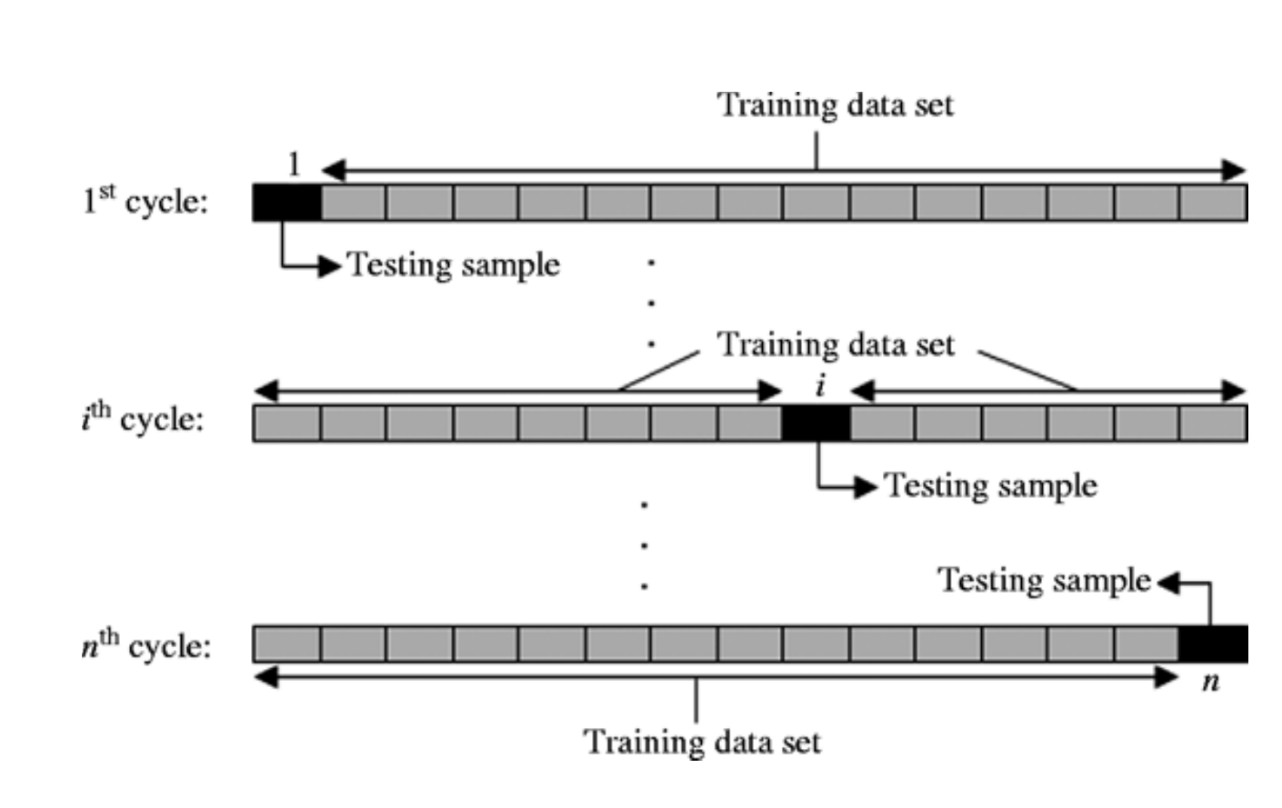
In [25]:
HTML("""
<h2>Evaluation of decoding</h2>Receiver operating characteristic (ROC)

    <center><embed src="{0}" height=400'></tr>

 """.format(figpath+ 'DT_1D_decoding_AUROC1.png'))
Out[25]:
In [26]:
HTML("""
 <h2>Evaluation of decoding</h2>Area under the ROC curve
    <center><table border="0" width=100%/>
    <tr height=100%/><embed src="{0}"  height=300'></tr>
    </table>
 """.format(figpath+ 'DT_AUROC.png'))
Out[26]:
Use of simple decoding methods for prosthetics
In [27]:
HTML("""
    <center><table border="0" width=100%/>
    <tr height=100%/><img src="{0}" width=290'></tr>
    </table>
 """.format(figpath+ 'conclude.png'))
Out[27]:
Some Python scripts
In [28]:
HTML("""
 <h2>Object oriented programming</h2>
 <textarea rows="28" cols="60">
class Cell:
    def __init__(self,spikeTime,barOnsetTime,baselineTime,params={}):
        self.parameters =
        self.spikeTime =
        self.barOnsetTime =
        self.trialOnsetTime =
        self.firingRate =

    #---------------------------------------------------------
    def eval_tuningDirOriTime(self,nbDir=12,nbOri=6):
    #----------------------------------------------------------
    def eval_firingRate(self,window=0.75/6.6*1000):
    #----------------------------------------------------------
    def eval_trialOnsetTime(self,baselineTime):
    #-----------------------------------------------------
    def plot_raster(self,experiment,condition):
    #--------------------------------------------------------
    def plot_meanfr(self,experiment,figsize=(4,2)):
    #---------------------------------------------------------
    def isDtTrajectory(self):
    #---------------------------------------------------------
    def meanFiringRate(self,exp):
    #------------------------------------------------------#
    def temporalTuningDT_fit(self,Nest=12):
    #------------------------------------------------------#

</textarea>
 """)
Out[28]:
In [29]:
HTML("""
<h2>Object oriented programming</h2>
<textarea rows="7" cols="100">
-> param ={"barSpeed":6.6,"tstart":0.,"tstop":2500.,"tbaseline" : 400.,"angleBin":30.}
-> V1DataObject = DataSetV1(pathToMatFolder)
-> cell_num = 6
-> cell = Cell(V1DataObject.spikeTime[cell_num],V1DataObject.tbar[cell_num],V1DataObject.parameters["tbaseline"],params)
-> c.plot_raster(experiment=0,condition=0,figsize=(6,4))
</textarea>
<img src="{0}" width=60%/>
""".format(figpath+ 'cell_response_c.png'))
Out[29]:
Object oriented programming
In [30]:
HTML("""
 <h2>Modeling and Statistics : numpy,scipy</h2>

<img src="http://latex.codecogs.com/gif.latex?\Large{ f(\Phi, \Theta, t) =
R_{0}+(R_m-R_{0})\cdot A(t)\cdot (b+(1-b)\cdot e^{\kappa_\theta\cdot(\cos(2(\theta-\phi_0))-1)}
\cdot e^{\kappa_\phi\cdot(\cos(\phi-\phi_0)-1)})}" border="0"/><p>
  <textarea rows="28" cols="60">
    def model_DirIndepOri(parsdict,Ndir,Nori):
        T=parsdict["T"]
        mA= parsdict['mA']
        sA= parsdict['sA']
        b = parsdict['b']
        R_min = parsdict['R_min']
        R_max = parsdict['R_max']
        theta0 = parsdict['theta0']
        k_o = parsdict['k_o']
        k_d = parsdict['k_d']
        #---------------------
        dirs = np.linspace(0, 2*np.pi, Ndir, endpoint=False)
        oris = np.linspace(np.pi/2,3*np.pi/2, Nori, endpoint=False)
        xv, yv = np.meshgrid (dirs,oris) #shape(Nori,Ndir),inversed
        #---------------------
        theta0 = theta0*np.pi/180.
        if k_o==0:
            f = np.exp(k_d*(-np.sin(xv-theta0)-1))
        else:
            f = np.exp(k_o*(np.cos(2*(yv-theta0))-1))
            f *= np.exp(k_d*(-np.sin(xv-theta0)-1))
        import matplotlib.mlab as mlab
        tc = np.zeros((Ndir,Nori,T))
        for t in range(T):
            A = mlab.normpdf(t,mA,sA)*np.sqrt(2*np.pi)*sA
            tc[:,:,t] = R_min + (R_max-R_min)*A*(b+(1-b)*f.transpose())
        return tc
 </textarea>
 """)
Out[30]:
Modeling and Statistics : numpy,scipy
In [31]:
HTML("""
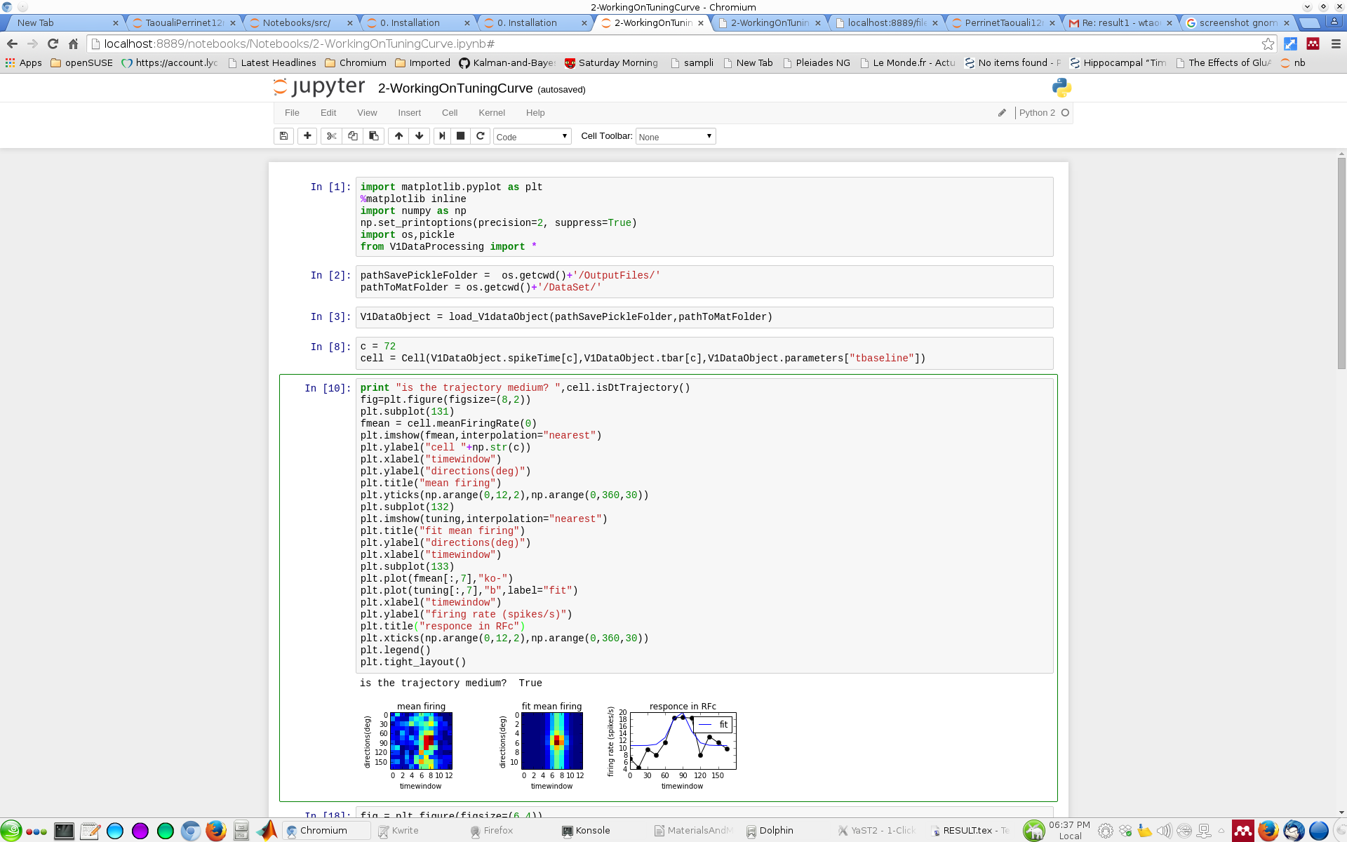
<h2>Ipython notebook + matplotlib</h2>
<img src="{0}" height=61%/>
""".format(figpath + 'snapshot1.png'))
Out[31]:
Ipython notebook + matplotlib
In [32]:
HTML("""
    <center>
    <h1>Thank you !!</h1>
    <h1>Questions??</h1>
    <table border="0" width=100%/>
    <tr height=100%/><img src="{0}" width=290 type='application/pdf'></tr>
    </table>
 """.format(figpath+ 'questions.png'))
Out[32]:
Thank you !!
Questions??

In [33]:
HTML("""
<h1 class="title">Decoding of feature selectivity in neural activity</h1>
<h1>Concrete applications in visual data</h1>
<h2>Wahiba Taouali, INMED - Laurent U Perrinet, INT</h2>
 <img src="{0}" height=61%/>
 """.format(figpath + 'troislogos.png'))
Out[33]:
Decoding of feature selectivity in neural activity
Concrete applications in visual data
Wahiba Taouali, INMED - Laurent U Perrinet, INT
Acknowledgements:
- PhD program: Anna Montagnini, Frédéric Chavane, Nadia Pittet, INT, Marseille
- Material: Peggy Series, Christopher Olah
- NeuroPhysiology: Giacomo Benvenuti, Frédéric Chavane, INT, Marseille