Edge co-occurrences can account for rapid categorization of natural versus animal images
Abstract
Making a judgment about the semantic category of a visual scene, such as whether it contains an animal, is typically assumed to involve high-level associative brain areas. Previous explanations require progressively analyzing the scene hierarchically at increasing levels of abstraction, from edge extraction to mid-level object recognition and then object categorization. Here we show that the statistics of edge co-occurrences alone are sufficient to perform a rough yet robust (translation, scale, and rotation invariant) scene categorization. We first extracted the edges from images using a scale-space analysis coupled with a sparse coding algorithm. We then computed the ``association field’’ for different categories (natural, man-made, or containing an animal) by computing the statistics of edge co-occurrences. These differed strongly, with animal images having more curved configurations. We show that this geometry alone is sufficient for categorization, and that the pattern of errors made by humans is consistent with this procedure. Because these statistics could be measured as early as the primary visual cortex, the results challenge widely held assumptions about the flow of computations in the visual system. The results also suggest new algorithms for image classification and signal processing that exploit correlations between low-level structure and the underlying semantic category.
A study of how people can quickly spot animals by sight is helping uncover the workings of the human brain.
Scientists examined why volunteers who were shown hundreds of pictures - some with animals and some without - were able to detect animals in as little as one-tenth of a second.
They found that one of the first parts of the brain to process visual information - the primary visual cortex - can control this fast response.
More complex parts of the brain are not required at this stage, contrary to what was previously thought.
). This is used to compute the chevron map in Figure~2.](/publication/perrinet-bednar-15/figure_model_hu_b59ceb4637730f86.webp)

![]()
![]()
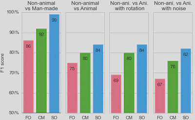
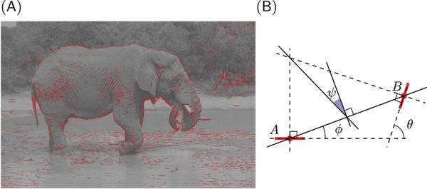
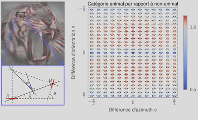
3, we used a standard Support Vector Machine (SVM) classifier to measure how each representation affected the classifier’s reliability for identifying the image category. For each individual image, we constructed a vector of features as either (FO) the histogram of first-order statistics as the histogram of edges’ orientations, (CM) the chevron map subset of the second-order statistics, (i.e., the two-dimensional histogram of relative orientation and azimuth; see Figure 2 ), or (SO) the full, four-dimensional histogram of second-order statistics (i.e., all parameters of the edge co-occurrences). We gathered these vectors for each different class of images and report here the results of the SVM classifier using an F1 score (50% represents chance level). While it was expected that differences would be clear between non-animal natural images versus laboratory (man-made) images, results are still quite high for classifying animal images versus non-animal natural images, and are in the range reported by\citet{Serre07} (F1 score of 80% for human observers and 82% for their model), even using the CM features alone. We further extend this results to the psychophysical results of Serre et al. (2007) in Figure 5.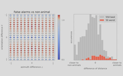
Communiqué de presse INSB : Comment nait la première impression d’une scène visuelle
En modélisant notre capacité à distinguer un animal dans une scène visuelle, des chercheurs de l’Institut de Neurosciences de la Timone et de l’Université d’Edinburgh lèvent le voile sur certains des mystères de la perception visuelle. Ils démontrent que la classification très rapide par le cerveau d’une image contenant ou non un animal, est possible à un niveau de représentation relativement primitif à partir de régularités statistiques simples, et non, comme cela est généralement admis, après une longue série d’analyses visuelles de plus en plus abstraites. Cette étude est publiée dans la revue Scientific Reports.
Classifier une image, par exemple en décidant si elle contient ou non un animal, est une des fonctions de base du cerveau. Dans le royaume animal, on comprend aisément qu’elle constitue une fonction vitale aussi bien pour des prédateurs que pour leurs proies. Les mécanismes sous-jacents sont de plus en plus étudiés aussi bien dans le domaine des systèmes d’intelligence artificielle que dans celui des Neurosciences, mais ils restent encore bien mystérieux pour les chercheurs. En effet, si les réseaux d’ordinateurs les plus avancés peuvent aujourd’hui aisément calculer numériquement des quantités phénoménales de données à partir de bases de données pharaoniques, même les systèmes les plus avancés de classification d’images n’égalent pas encore les capacités d’un jeune enfant!
Laurent Perrinet de l’Institut de Neurosciences de la Timone à Marseille et James Bednar de l’université d’Edinburgh en Écosse, ont modélisé la façon dont nous pouvons classer différentes catégories d’images. Leur l’objectif initial était de différencier des scènes visuelles naturelles de scènes d’intérieur, mais ils ont pu montrer que ce système simple de classification permettait aussi de détecter en une fraction de seconde des animaux dans une image. En effet, ils ont mis en évidence qu’un niveau de performance comparable à celui d’observateurs humains est atteignable tout en utilisant un niveau de représentation très primitif, et non, comme cela est généralement admis, après une longue série d’analyses visuelles de plus en plus abstraites (détection des yeux et des membres, puis de la tête et du corps, etc…).
Cette représentation primitive se base sur les modèles existants de représentation des images dans les aires visuelles de bas niveau des primates. On estime en effet que dans le cortex visuel primaire les images visuelles sont représentées dans l’activité neurale comme l’organisation de contours élémentaires, à la manière d’un peintre qui dessine une silhouette en une série de coups de pinceau. Une des innovations majeures dans cette étude consiste à simplement utiliser la fréquence des configurations entre des paires de contours élémentaires comme représentation d’entrée utilisée pour le classificateur.
Pour arriver à ce résultat, les chercheurs ont utilisé des modèles mathématiques de la représentation des images dans le cortex visuel primaire et en particulier les inter-relations entre des éléments de contours voisins. En étudiant les résultats de l’analyse, on note que dans les images naturelles, des contours parallèles sont observés majoritairement, signe que les contours et textures présents dans les images contiennent en majorité des alignements. C’est encore plus vrai dans les environnements artificiels comme dans une scène d’intérieur (par exemple un bureau) où les bords francs dominent. On montre aussi que les objets co-circulaires (c’est-à-dire des configurations symétriques) sont aussi relativement plus présents que des configurations aléatoires.
La principale nouveauté de cette étude est de montrer que les images contenant un animal (quelle que soit son espèce ou sa position dans l’image) contiennent sensiblement plus de configurations symétriques. Cette différence suffit pour expliquer le niveau de performance de classification chez les humains quand on leur présente de telles scènes de façon très brève.
Pour valider cette hypothèse, les chercheurs ont alors utilisé des données précédemment enregistrées dans lesquelles des volontaires regardaient et classifiaient des centaines d’images. En utilisant cette représentation primitive, ils ont mis en évidence qu’un programme très simple pouvait facilement classifier les images comme contenant ou non un animal, sans avoir besoin d’une connaissance plus élaborée sur les caractéristiques de l’animal comme sa position, sa taille ou son orientation sur l’image.
Cette découverte peut accélérer le développement de requêtes via des images dans les moteurs de recherche, comme Google et Facebook, car elle permet une classification simple et robuste grâce à des caractéristiques statistiques de bas niveau basées sur la géométrie des objets. Elle pourrait ainsi améliorer l’efficacité de tels algorithmes. Toutefois, et comme cela a été mis en évidence dans la psychophysique humaine, les catégories visuelles doivent être visuellement assez distinctes: ce traitement rapide ne permet pas, par exemple, de distinguer une scène de montagne d’une scène de mer. De manière surprenante, les chercheurs ont montré que lorsque les humains se trompent en classifiant de manière erronée une image comme contenant un animal, le programme a tendance à se tromper de la même façon! En utilisant des modèles mathématiques, on peut donc imaginer synthétiser des images d’animaux qui en fait, n’en contiendraient pas. Ces “chimères” seront sûrement très utiles pour percer encore plus les mystères du système visuel.
Dans le futur, l’extension de cette représentation calculée sur l’ensemble de l’image pourrait être améliorée en la couplant à des processus de classification locaux permettant de déterminer par exemple la position de l’objet à classifier et de segmenter progressivement la figure du fond afin de diminuer ainsi les distractions.
Laurent U Perrinet
Researcher in Computational Neuroscience
My research interests include Machine Learning and computational neuroscience applied to Vision.